
Introduction
Building on the work we did in the previous post, I spent today building a normal SABR volatility surface for BTC options, with the end-goal of pricing inverse options on Deribit (which will be in the next post). This post is about what actually mattered, what broke repeatedly, and what finally made the model behave. This is not a SABR tutorial. It is about scaling, units, and why crypto makes you pay attention to things that rate quants get for free!
My Choice of Model
Bitcoin options are quoted in implied volatility, but the underlying is a large positive price level, not a rate or a yield. Let’s set some notation:
be the BTC spot price at time
be the forward price of BTC for maturity
be the option strike
be time to expiry in years

Working in Black lognormal volatility assumes dynamics proportional to 

- convexity effects
- sensitivity to extrapolation
- numerical instability in the wings
This is especially relevant for BTC, where 
A normal (Bachelier) volatility, quoted in USD per 
This motivates using normal SABR, with the elasticity parameter fixed to zero: 
Vol-of-Vol Is Tiny
In normal SABR with 

where:
is the SABR volatility level parameter, with units USD per
is the volatility of volatility parameter
For BTC we have these sorts of numbers:
- In the wings,
or more
- Therefore
is on the order of


Which means if one naively sets (as I did):


then
For BTC in USD price units, 
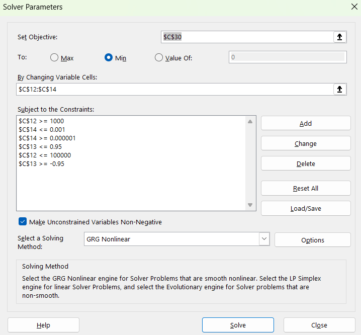
This was the single most important fix. So my Solver Parameters were set like this. For a particular time to expiry, in cell C12 was alpha (which had to be strictly greater than 1000 so that it didn’t find the local minimum created at 


Why Relative SSE was Essential?
Market normal vols for BTC are on the order of 


produces objective values in the billions, which is numerically bad to optimisers like the Excel Solver.
Instead, the calibration objective was defined as a relative squared error:

where:
indexes strikes or moneyness points
are user-chosen weights
are market normal vols
are model normal vols
This produces a dimensionless objective of order 
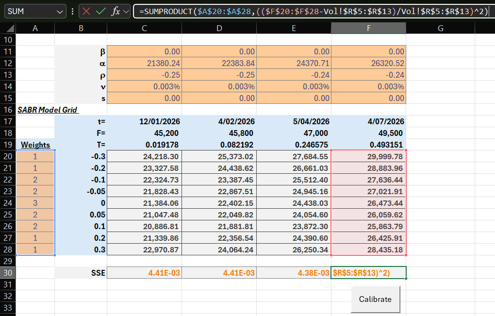
So you can see here in my SSE formula, I use the relative SSE variant, where I have divided by the market quotes (in cells Vol!$R$5:$R$13):
The Role of Weights
When calibrating a parametric volatility surface, the objective function is not uniquely defined. The choice of weights determines which parts of the smile the model is incentivised to fit accurately, and which parts it is allowed to smooth over.
In this calibration, the objective function takes the form:

- where
The weights
Since BTC volatility smiles are quite noisy in the wings, and often quoted with lower liquidity far from ATM, the smile is highly sensitive to small data errors when working in price units.
If all points are given equal weight, the Solver will often overfit noisy wing points, distort curvature to reduce a few large absolute errors, and sacrifice ATM stability to chase illiquid strikes.
This is especially problematic when the vols are large (
The weights are applied as a simple function of moneyness, and the exact numbers are not special. What matters more is the ordering, which simply reflects three facts:
- ATM options are the most liquid
- ATM vols dominate pricing and hedging
- Wing quotes contain more noise and less information
The Role of the Shift Parameter
When working with log-moneyness, the expression

implicitly assumes:
- stable behaviour as


While BTC prices are strictly positive, inverse options and payoff transformations naturally involve expressions in 
To address this, a shift parameter 
Shifted Log-Moneyness
We define the shifted forward and shifted strike to be:


where:
is a shift parameter, expressed in USD
The shifted log-moneyness is then defined as:

This replaces 
Note that:
- when
, this reduces to standard log-moneyness
- when
, low strikes are pushed away from zero
- the mapping between
and
How the Shift Enters the SABR Calibration
The SABR model itself does not change, all parameters remain the same. Instead, it is how the strikes are generated and interpreted. When we are given now log-moneyness 


which makes the smile parameterised in shifted log-moneyness and the model should still behave nicely in the wings. But most importantly, the calibration model should be compatible with inverse-payoff transformations (next blog).
Note that the shift parameter
Calibration Results
For now, just to get the calibration working, we will use a null shift parameter.
Here are the results:
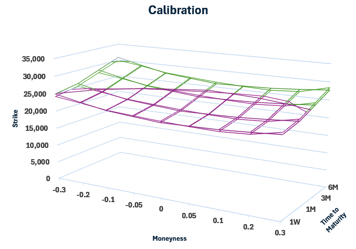
The surface plot above shows the calibrated normal SABR volatility surface alongside the corresponding market-quoted normal volatilities, using a null shift parameter. The model reproduces the observed term structure and smile shape across all quoted maturities, with particularly close agreement around the ATM region where liquidity is highest. Deviations between the model and market surfaces are small relative to the overall volatility level and exhibit no systematic structure, indicating that the calibration is capturing the dominant features of the smile rather than overfitting local noise.
Importantly, the fitted parameters vary smoothly across maturities, and the resulting surface is well behaved in both moneyness and time. This confirms that normal SABR with
Shifted-SABR
Normal SABR does not require a shift for mathematical validity. The model already accommodates negative values cleanly.
A shift
- working in log-moneyness
- transitioning to Black-style implied volatilities
- building a unified framework compatible with inverse or lognormal conventions
At this stage, the shift is set to 
Why inverse BTC options change the problem
The ultimate goal is to price inverse BTC options on Deribit. These options:
- Settle in BTC
- Have payoffs that are non-linear in the BTC price
- Cannot be priced correctly by plugging a normal or Black vol into a standard USD-settled formula
This means the next step is not modifying SABR further, but rather building a pricing layer that respects:
- the inverse payoff
- the underlying variable transformation
- Deribit’s implied volatility convention
Only once prices are correct does it make sense to introduce shifted moneyness or shifted SABR.
Conclusion
What I discovered in this exercise is that SABR itself is not fragile, the units are!
Once the scale is correct, normal SABR works extremely well for BTC. Most issues arise from importing intuition from rates or equities without adjusting for the fact that the underlying is a fifty-thousand-dollar asset, not a five-percent yield.
With a stable normal SABR surface calibrated to a synthetic market grid, the next step is to replace that grid with real Deribit market quotes, and to extend the framework to include a shift parameter in a controlled way.
This section outlines how those two steps will be done.
Appendix
The SABR calibration is automated using a small VBA layer that wraps Excel’s Solver and applies it consistently across maturities. For each expiry, the code constructs a relative least-squares objective based on weighted differences between model and market normal volatilities, and then minimises this objective by adjusting the SABR parameters 


Option Explicit

'===========================================================
' Shifted SABR Normal (Bachelier) implied vol approximation.
'
' Written by: Benjamin Whiteside
' Last Modified: 06/01/2026
'
' Hagan-style normal SABR on shifted F,K:
'   Ft = F + shift, Kt = K + shift
'
' Returns normal vol in same price units as F,K (e.g. USD / sqrt(year)).
'
' Signature:
'   SABR_N_Shift(F, K, T, alpha, beta, rho, nu, shift)
'
' Notes:
' - Uses ATM expansion when |Ft-Kt| is tiny to avoid 0/0.
' - Assumes T in years (ACT/365 or your chosen convention).
' - Requires alpha>0, nu>=0, |rho|<1.
'===========================================================

Public Function SABR_N_Shift( _
    ByVal F As Double, _
    ByVal K As Double, _
    ByVal T As Double, _
    ByVal alpha As Double, _
    ByVal beta As Double, _
    ByVal rho As Double, _
    ByVal nu As Double, _
    ByVal shift As Double) As Double

    On Error GoTo FailFast

    ' --- Basic guards
    If T <= 0# Then
        SABR_N_Shift = 0#
        Exit Function
    End If
    If alpha <= 0# Then
        SABR_N_Shift = CVErr(xlErrNum)
        Exit Function
    End If
    If nu < 0# Then
        SABR_N_Shift = CVErr(xlErrNum)
        Exit Function
    End If
    If rho <= -0.999999 Or rho >= 0.999999 Then
        SABR_N_Shift = CVErr(xlErrNum)
        Exit Function
    End If
    If beta < 0# Or beta > 1# Then
        SABR_N_Shift = CVErr(xlErrNum)
        Exit Function
    End If

    Dim Ft As Double, Kt As Double, d As Double
    Ft = F + shift
    Kt = K + shift
    d = Ft - Kt

    ' If beta>0 we will use powers of Ft, Kt, so they must be positive
    If beta > 0# Then
        If Ft <= 0# Or Kt <= 0# Then
            SABR_N_Shift = CVErr(xlErrNum)
            Exit Function
        End If
    End If

    ' ATM threshold: relative to scale of prices
    Dim atmTol As Double
    atmTol = 0.0000001 * (1# + Abs(Ft) + Abs(Kt))

    ' ---------- ATM branch ----------
    If Abs(d) < atmTol Then
        SABR_N_Shift = SABR_N_ATM(Ft, T, alpha, beta, rho, nu)
        Exit Function
    End If

    ' ---------- Non-ATM branch ----------
    Dim FK As Double, A As Double
    FK = Ft * Kt

    ' For beta not 0, FK must be positive (powers). With shift it should be.
    If beta <> 0# Then
        If FK <= 0# Then
            SABR_N_Shift = CVErr(xlErrNum)
            Exit Function
        End If
    End If

    A = PowSafe(FK, (1# - beta) / 2#)

    Dim z As Double, xz As Double
    z = (nu / alpha) * A * d

    xz = XofZ(z, rho)

    ' Strike correction B
    Dim oneMinusB As Double
    oneMinusB = 1# - beta

    Dim Bcorr As Double
    Bcorr = 1# _
        + (oneMinusB * oneMinusB / 24#) * (d * d / PowSafe(FK, 1# - beta)) _
        + (oneMinusB ^ 4 / 1920#) * (d ^ 4 / PowSafe(FK, 2# - 2# * beta))

    ' Time correction C
    Dim Ccorr As Double
    Ccorr = ( _
        (oneMinusB * oneMinusB / 24#) * (alpha * alpha / PowSafe(FK, 1# - beta)) _
        + (rho * beta * nu * alpha / (4# * PowSafe(FK, (1# - beta) / 2#))) _
        + ((2# - 3# * rho * rho) / 24#) * (nu * nu) _
    ) * T

    ' Main normal vol formula:
    ' sigmaN = alpha*(FK)^(beta/2) / Bcorr * (z/x(z)) * (1 + Ccorr)
    Dim pre As Double, ratio As Double
    pre = alpha * PowSafe(FK, beta / 2#) / Bcorr

    ' z/xz tends to 1 as z->0, but we're not ATM here; still, be safe:
    If Abs(xz) < 1E-16 Then
        ratio = 1#
    Else
        ratio = z / xz
    End If

    SABR_N_Shift = pre * ratio * (1# + Ccorr)
    Exit Function

FailFast:
    SABR_N_Shift = CVErr(xlErrValue)
End Function


'===========================================================
' ATM normal-vol expansion (shifted already applied, input is Ft)
' sigma_ATM = alpha * Ft^beta * (1 + [ ... ] * T)
'===========================================================
Private Function SABR_N_ATM( _
    ByVal Ft As Double, _
    ByVal T As Double, _
    ByVal alpha As Double, _
    ByVal beta As Double, _
    ByVal rho As Double, _
    ByVal nu As Double) As Double

    Dim oneMinusB As Double
    oneMinusB = 1# - beta

    ' Handle beta=0 cleanly: Ft^beta = 1
    Dim FtPowBeta As Double
    FtPowBeta = PowSafe(Ft, beta)

    Dim term As Double
    term = ( _
        (oneMinusB * oneMinusB / 24#) * (alpha * alpha / PowSafe(Ft, 2# - 2# * beta)) _
        + (rho * beta * nu * alpha / (4# * PowSafe(Ft, 1# - beta))) _
        + ((2# - 3# * rho * rho) / 24#) * (nu * nu) _
    ) * T

    SABR_N_ATM = alpha * FtPowBeta * (1# + term)
End Function


'===========================================================
' x(z) helper for SABR (Hagan)
' x(z) = ln( (sqrt(1 - 2*rho*z + z^2) + z - rho) / (1 - rho) )
' For small z, use series x(z) ~ z to avoid precision loss.
'===========================================================
Private Function XofZ(ByVal z As Double, ByVal rho As Double) As Double
    Dim absz As Double
    absz = Abs(z)

    If absz < 0.00000001 Then
        ' For tiny z, x(z) ~ z (sufficient; prevents 0/0 noise)
        XofZ = z
        Exit Function
    End If

    Dim inside As Double, num As Double, den As Double
    inside = 1# - 2# * rho * z + z * z
    If inside < 0# Then
        ' Numeric guard (shouldn't happen for real params)
        inside = 0#
    End If

    num = Sqr(inside) + z - rho
    den = 1# - rho

    If num <= 0# Or den <= 0# Then
        ' Fallback: if expression is numerically bad, approximate with z
        XofZ = z
    Else
        XofZ = Log(num / den)
    End If
End Function


'===========================================================
' Safe power: handles x^p for x>0, and x=0 for p>0
' For negative x and non-integer p, returns error by raising.
'===========================================================
Private Function PowSafe(ByVal x As Double, ByVal p As Double) As Double
    If x = 0# Then
        If p > 0# Then
            PowSafe = 0#
            Exit Function
        Else
            Err.Raise vbObjectError + 513, , "PowSafe: 0 to non-positive power"
        End If
    End If

    If x < 0# Then
        ' Only allow integer powers for negative base
        If Abs(p - CLng(p)) > 0.000000000001 Then
            Err.Raise vbObjectError + 514, , "PowSafe: negative base with non-integer power"
        End If
    End If

    PowSafe = x ^ p
End Function
Final Implementation Notes in VBA & Numerical Considerations
The SABR implementation applies the shift at the level of the forward and strike, defining 


The code confirms numerical stability by separating the ATM and non-ATM regimes. When the shifted forward and strike are close, the implementation switches to the analytic ATM expansion to avoid the 

