A Recipe for Pricing

Introduction

In this blog we will be looking at the Recipe for Pricing.

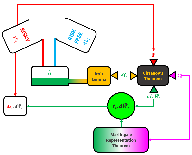
The recipe involves starting by mixing together a risky asset and a risk-free asset. Then we take that mixture and feed it into the Ito’s Lemma machine. Out of that machine pops the stochastic differential equation for the mixture. Then we throw that mixture in the Girsanov oven, together with the original real-world probability measure $\mathbb{P}$ . Let it cook for 30 minutes at 180 degrees celsius and out comes a new risk-neutral probability measure $\mathbb{Q}$ and the cooked mixture $d\widetilde{f}_t$ and $\widetilde{W}_t$ .

With these cooked ingredients we then cool it by placing it in the Martingale Representation Theorem. When it is cooled thoroughly, the cooked mixture reduces to $f_t$ . Then all we need to do it put the icing on it by substituting everything back in to the original stochastic differential equation for the risky asset, but now with a new, cooked-up Wiener process $d\widetilde{W}_t$ .

So let’s see how this recipe works.

The Black-Scholes Pricing Framework

Risky assets are assets whose value changes randomly. From one instant to the next its price might move up some amount, or down some amount. It could even stay the same. The direction and the amount of movement is random.

So how do we price such risky assets?

Well, we need to introduce some assumptions. Different sets of assumptions define different so-called pricing frameworks. One very popular framework is the Black-Scholes (BS) pricing framework (also known as the Black-Scholes Model), but there are others. Under the BS framework there are 7 assumptions. We won’t go in to them here suffice to point out that one of the assumptions is: the log return of a risky asset price is a random walk with drift. Another way to say this is: risky asset prices follow a geometric Brownian motion.

It turns out that this is a pretty good assumption because GBMs exhibit quite a few similarities with what is observed in real life. For example, and this one is fairly simple: a GBM only assumes positive values, just like real (risky) stock prices! Another similarity is that the amount of ‘roughness‘ as seen in the graph of a GBM is about the same amount of ‘roughness‘ as seen in the graph of a risky stock price.

However, GBMs are not a perfect replication of reality. For example, the volatility of risky stock prices in real life changes over time, even randomly. But the volatility of a GBM is constant over time. Moreover, real life stock prices exhibit jumps caused by unpredictable events, but GBMs are continuous.

Never-the-less the Black-Scholes model is a very popular model in quantitative finance and can be used to accurately predict the price of a risky (random) asset; and in this article we will see just how this is done in practice.

First of all, we must operate under the so-called Black-Scholes-Merton framework (or the BSM model). We certainly don’t have to use the BSM model and, in fact, there are a great many other frameworks we could use. Some frameworks (like the Black-76 framework) contains different assumptions that might better suit some other risky asset that refuses to play by the rules of the Black-Scholes framework (for example, commodity futures). But there are risky assets which do play by the Black-Scholes-Merton rules quite well, and it is these which we will focus our attention on in this article.

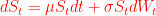
The BSM Model assumes that the price of a risky asset follows a geometric Brown motion with drift. This means that the change in price of risky assets is equal to some amount of drift (up or down) plus some amount of randomness (the size of the up or down movement). The combination of the drift and the amount of randomness can be captured, or represented, by the following equation:

$\displaystyle\text{Change in Price} = \text{Drift}+\text{Volatility}$

But what good is knowing the change of the price? Isn’t it better to know what the actual price is?

That’s a good question, but defining actual prices is a little too specific. We would prefer a generalised approach to pricing and not tie ourselves to any sort of value magnitude or type (like different currencies). You see, a change in price is a dimensionless ratio and is much easier to manipulate and apply to an asset (like, simply multiplying it). Plus, using some sophisticated tools, we will be able to convert a change in price to an actual price anyway.

Let’s put some standard mathematical symbols to our heuristic equation above. I have coloured this equation red to indicate that it is for the risky asset:

$dS_t = \mu S_t dt + \sigma S_t dW_t$

Here, $t$ denotes the passage of time, $S_t$ denotes the risky asset price, $\mu$ is the drift percentage and $\sigma$ is the volatility percentage. What makes this equation geometric is the factor of $S_t$ in the drift and the volatility.

Sometimes you’ll see this equation written divided through by the spot price $S_t$ like so:

$\frac{dS_t}{S_t} = \mu dt + \sigma dW_t$

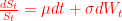
but the former is more common, mostly to indicate its geometric property.

This equation looks like your typical differenial equation except for that $dW_t$ at the end there. This is the rate of change of Brownian motion (hence the name); and it makes the equation a stochastic differential equation, or SDE for short.

As mentioned before, the rate of change of the price of the risky asset $dS_t$ , although general, doesn’t do us much good when it comes to find the actual physical price. We need the actual price, denoted $S_t$ ; and the actual price today would be denoted with a $t=0$ , i.e. by $S_0$ .

It is very difficult to take a randomly evolving thing and create something specific (like an actual price) from it. But it turns out we can with the help of a few mathematical tools and another asset: the risk-free asset.

By incorporating a risk-free asset in with a risky asset to annihilate randomness was a key insight in to the Black-Scholes-Merton framework of 1973.

So the theme for the rest of the article is to derive an actual price $S_t$ given just the 7 assumptions of the BSM model and the stochastic differential equation expressing the rate of change of a risky asset.

What else do we need to assume?

The next assumption we need from the BSM model to be able to make any progress in our quest is the one that states that the rate of return of a risk-free asset is constant, a reasonable assumption. This has a stochastic differential equation representation too, and I’ve coloured this one blue to indicate that it is risk free:

$dB_t = r_t B_t dt$

Where $B_t$ is the value of the risk-free asset at time $t$ , and $r_t$ is the so-called risk-free interest rate. Note that this equation has no random component, i.e. there is no $dW_t$ part.

As it turns out, by defining such an object in the BSM model, allows us to discount the risky asset price from any future time $t$ back to today $t=0$ by the risk-free rate. This is referred to as discounting by the risk-free rate. Furthermore, this assumption allows us to utilise continuous discounting, which means we can define

$\displaystyle\text{Discounted Value} := \int_0^T e^{-\lambda t}\left[\text{Future Value}\right]dt$

Continuous discounting and the exponential

Why is continuous discounting represented by the exponential $e^{-\lambda t}$ , you may wonder?

Suppose you begin with $m_0$ amount of money at time $t=0$ and there is some length of time $T$ that you hold that money for, during which time it accrues interest.

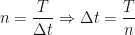
One thing you could do is to divide that length of time up in to smaller pieces (a method known as discretisation), each with a length of time $\Delta t$ ; and over each one of these smaller time periods we will apply a small interest rate $\latex r$, causing a small increase in the amount of money you have, $\Delta m$ :

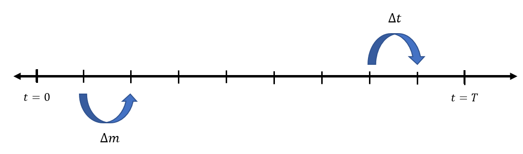
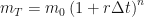
How many small intervals of $\Delta t$ are there? Well, that is equal to the total length $T$ divided by the length of the smaller intervals $\Delta t$ , thus the number of small intervals is:

$\displaystyle n = \frac{T}{\Delta t} \Rightarrow \Delta t = \frac{T}{n}$

What interest rates do, is this: they create a change in money amount $\Delta m$ by taking an interest rate $r$ , scaling it by the time interval $\Delta t$ , and then multiplying all of that by the amount of money you have $m$ . The formula for this growth action on the initial amount of money is, very simply, the product of all these little actions:

$\displaystyle \Delta m_0 = r \times \Delta t \times m_0$

Thus, an initial amount of money $m_0$ will grow by an amount $\Delta m_0$ , i.e.

$\displaystyle m_1 = m_0 + \Delta m_0$

which equals

$\displaystyle m_1 = m_0 + r\Delta t m_0$

factoring out the initial amount of money $m_0$ gives

$\displaystyle m_1 = m_0(1+r\Delta t)$

Then, for each little time step $\Delta t$ we are simply going to keep performing this mapping of taking the money from the previous time step, and multiplying it by a factor of $1+r\Delta t$ , over and over again, precisely $n$ times, until we hit $T$ .

Since multiplication commutes, this means that for $n$ time steps, we will have $n$ factors of $1+r\Delta t$ , thus:

$\displaystyle m_T = m_0 \left(1+r \Delta t\right)^n$

We already know what $\Delta t$ is (above), so we can substitute that in:

$\displaystyle m_T = m_0 \left(1+ \frac{rT}{n}\right)^n$

Now we need to un-discretise time, and the way we do this is to apply the limit as $n \rightarrow \infty$ , i.e. see what happens to $m_T$ as we increase the number of time steps to infinity.

$\displaystyle m_T = m_0 \lim_{n\rightarrow\infty} \left(1+ \frac{rT}{n}\right)^n$

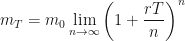
If we make the substitution $rT = y$ , then we get

$\displaystyle m_T = m_0 \lim_{n\rightarrow\infty} \left(1+ \frac{y}{n}\right)^n$

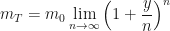
and then a second substitution $x = \frac{n}{y}$ , then we get

$\displaystyle m_T = m_0 \lim_{x\rightarrow\infty} \left(1+ \frac{1}{x}\right)^{xy}$

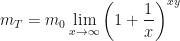
then using the property of exponents to split the exponent up, we get

$\displaystyle m_T = m_0 \lim_{x\rightarrow\infty} \left[\left(1+ \frac{1}{x}\right)^{x}\right]^{y}$

and now, the part in brackets – together with the limit, is well-known to be $e$ .

$\displaystyle m_T = m_0 e^y$

Finally, we need to reverse our subsitutions:

$\displaystyle m_T = m_0 e^y = m_0 e^{rT}$

as required.

Combining a Risky Asset with Risk-a Free Asset

By continuously discounting at the risk-free interest rate we have essentially defined a new function $f$ by the product of a risk-free asset and a risky asset, which I’ll show as green to indicate that it is a mixture of the two:

$\displaystyle f:= Se^{-\int_0^t r_u du}$

As written, this function is also random and contains drift (both properties of risky things) because it contains a factor of $S_t$ and hence contains Brownian motion; and, as much as we’d like to, we can’t just write:

$S = f e^{\int_0^t r_u du}$

as this gives us no information because the right-hand side still contains $f$ .

As before, let’s look at the change in $f$ , i.e. let’s see if we can derive $df$ .

It’s difficult to take the derivative of a random function. But luckily we can use Itô’s Lemma (which is basically the random, stochastic version of the chain rule) to perform the mapping

$\displaystyle f \mapsto df$

So let’s look at how we do that…

Practical Itô’s Lemma

Once you have a composite function like $f$ you can apply Itô’s lemma to derive its derivative $df$ . The formula for doing this is:

$\displaystyle df = \partial_t fdt + \partial_S fdS_t + \frac{1}{2}\partial_{tt}fdt^2 + \frac{1}{2}\partial_{SS}fdS_t^2 + \mathcal{O}(t,S_t)$

which is really just a sum of four parts and is derived from the Taylor series expansion of $df$ which looks like this:

$\displaystyle dS_t = \frac{\partial S_t}{\partial t}dt + \frac{\partial S_t}{\partial S_t}dS_t + \frac{1}{2!}\frac{\partial^2 S_t}{\partial t^2}dt^2 + \frac{1}{2!}\frac{\partial^2 S_t}{\partial S_t^2}dS_t^2 + \mathcal{O}(t, S_t)$

Both of these expansions are worth memorising if you are going to be doing a lot of these kinds of calculations.

But now we have to do some maths…

1st Part

The first part involves the calculation of the partial derivative of $f$ with respect to time $t$ . But first, let us make the notation a little easier to handle by defining the function of $x$ as the exponent:

$\displaystyle x(t) := \int_0^t -r(u)du$

Then, recalling the fundamental theorem of calculus, we immediately have that

$\displaystyle x^{\prime}(t) = \frac{d}{dt} \int_0^t -r(u)du = -r(t)$

which will be a useful result for us in just a second.

Right, let’s jump in and perform this partial derivative. The only explicit $t$ appears in the exponent and the variable $S$ is considered constant with respect to this partial derivative, hence:

$\displaystyle \partial_t f = \frac{\partial}{\partial t} \left( S e^{x(t)}\right) = x^{\prime}(t)S e^{x(t)} = -r(t)Se^{x(t)} = -r(t)f$

2nd Part

The second part is much easier. We just take the partial derivative of $f$ with respect to $S$ . There is only one explicit $S$ and the exponential is considered constant, hence:

$\displaystyle \partial_S f = \frac{\partial}{\partial S} Se^{x(t)} = e^{x(t)}$

3rd Part

The third part is always trivial because

$\displaystyle dt^2 = 0$

4th Part

The final and fourth part involves calculation of the second partial derivative of $f$ with respect to $S$ . In this case, we can take the result of the 2nd part and just take the partial derivative once more to obtain:

$\begin{aligned}\partial_{SS} &= \frac{\partial^2 f}{\partial S^2} \\ &= \frac{\partial}{\partial S} e^{x(t)} \\ &= 0\end{aligned}$

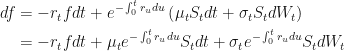
Combining Parts for Ito’s Lemma

This gives:

$\begin{aligned}df &= -r_t f_t dt + e^{-\int_0^t r_u du}dS_t + 0 + 0 \\ &= -r_t f_t dt + e^{-\int_0^t r_u du}dS_t\end{aligned}$

Now we need to substitute back in our original equation for $dS_t$ :

$\begin{aligned}df &= -r_t f dt + e^{-\int_0^t r_u du}\left(\mu_t S_t dt + \sigma_t S_t dW_t\right) \\ &= -r_t f dt + \mu_t e^{-\int_0^t r_u du} S_t dt + \sigma_t e^{-\int_0^t r_u du} S_t dW_t\end{aligned}$

We can’t go any further until we rearrange $f = e^{-\int_0^t r_u du} S_t$ in to

$\displaystyle S_t = f e^{\int_0^t r_u du}$

and notice that the negative exponent has now become a positive one. Now,

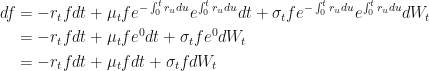
$\begin{aligned}df &= -r_t f dt + \mu_t f e^{-\int_0^t r_u du} e^{\int_0^t r_u du} dt + \sigma_t f e^{-\int_0^t r_u du} e^{\int_0^t r_u du} dW_t \\ & = -r_t f dt + \mu_t f e^0 dt + \sigma_t f e^0 dW_t \\ &= -r_t f dt + \mu_t f dt + \sigma_t f dW_t\end{aligned}$

and, collecting like terms to factor out the $dt$ we obtain:

$\displaystyle df = (\mu_t - r_t) f dt + \sigma_t f dW_t$

Rearrange to get dW Alone

The next step, is to get the above equation in to the right form.

Think about what we are going to do next: we are going to use Girsanov’s theorem to make an argument about $dW_t$ . Thus, $dW_t$ should be isolated and by itself – nothing out the front of it. In this step we ensure this by factoring out any coefficient of $dW_t$ . In our case we have this factor of $\sigma_t f$ , so we factor it out:

$\displaystyle df = \sigma_t f \left(\frac{\mu_t - r_t}{\sigma_t} dt + dW_t\right)$

and now the $dW_t$ component is isolated and we can implement Girsanov’s theorem.

Using Girsanov’s Theorem

Finding Lambda

Girsanov’s theorem is a theorem about $dW_t$ and about $\lambda$ . What is $\lambda$ ? Well, $\lambda$ is the coefficient of $dt$ that occurs when you do the re-arranging step we did above. It’s easy to define once $dW_t$ is isolated by factoring, and for our example is it just

$\displaystyle \lambda := \frac{\mu_t - r_t}{\sigma_t}$

What about the $\sigma_t f$ common to both $dt$ and to $dW_t$ ?

Well, it’s not really about the pieces common to both. The parameter $\lambda$ is just the coefficients relating to the $dt$ part, that’s it. I guess you could just divide both sides by that and it really doesn’t feture on the right-hand side anymore.

So, once we have found lambda we can implement Girsanov’s Theorem. How do we do that?

Well, it is pretty much just writing down the same paragraph. Every time you do this step, you’ll be stating the same thing over and over again without ever changing anything, so it is worth memorising it. I have, and now I know that when I get to this stage, I just blurt it out, word-for-word, without thinking. It’s needed though, and it’s important, because you can’t proceed to the next step unless you have clearly stated it. So let’s do it:

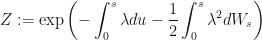
By Girsanov’s Theorem there exists an equivalent martingale measure (EMM) $\mathbb{Q}$ on the filtration $\mathcal{F}_t$ defined by the Radon-Nikodym derivative

$\displaystyle Z := \exp\left( -\int_0^s \lambda du - \frac{1}{2}\int_0^s \lambda^2 dW_s \right)$

such that under the measure $\mathbb{Q}$ , the stochastic process $\widetilde{W}$ is a $\mathbb{Q}$ -standard Wiener process and is

$\displaystyle \widetilde{W}_t = W_t + \int_0^t \lambda_u du$

or,

$\displaystyle dW_t = d\widetilde{W}_t - \lambda_t dt$

…by differentiating both sides with respect to $t$ .

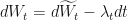
That’s it. This theorem only requires that we have defined precisely what $\lambda$ is (which is why we went to all the trouble of factoring everything out so we could find it!), the filtration is given right at the beginning when we defined our probability space, and this theorem simply produces a new probability measure $\mathbb{Q}$ , an a new Wiener process $\widetilde{W}$ on the new measure (it’s obviously not a Wiener process on the original probability measure $\mathbb{P}$ ).

The Martingale Representation Theorem

Now that we have been handed the new Wiener process $\widetilde{W}_t$ by Girsanov, what do we do with it?

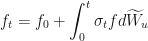
Ultimately, we have a stochastic process $f$ , and we know $df$ by virtue of Ito’s lemma. But these processes are Wiener processes under the original probability measure $\mathbb{P}$ . We need the equivalent process, say $\widetilde{f}$ , which is Wiener under the new probability measure $\mathbb{Q}$ !

The martingale representation theorem comes to the rescue, because it provides the stochastic process $\widetilde{f}$ so long as you have a driftless one in the first place.

OK, so what do we have? Our stochastic process (under $\mathbb{P}$ ) looks like this so far:

$\displaystyle df = \sigma_t f \left(\frac{\mu_t - r_t}{\sigma_t} dt + dW_t\right)$

This is certainly not driftless. Just look at that almighty drift as the coeffcient of the $dt$ term.

OK, let’s see what this stochastic process looks like under $\mathbb{Q}$ using the results from Girsanov’s theorem. We begin by substituting in $dW_t = d\widetilde{W}_t - \lambda_t dt$ ,

$\begin{aligned}d\widetilde{f} &= \sigma_t f \left(\frac{\mu_t - r_t}{\sigma_t} dt + dW_t\right) \\ &= \sigma_t f \left(\frac{\mu_t - r_t}{\sigma_t} dt + d\widetilde{W}_t - \lambda_t dt\right)\end{aligned}$

Let’s throw in what $\lambda_t$ equals:

$\displaystyle d\widetilde{f} = \sigma_t f \left(\frac{\mu_t - r_t}{\sigma_t} dt + d\widetilde{W}_t - \left( \frac{\mu_t - r_t}{\sigma_t} \right) dt\right)$

The lambda’s cancel out, and we are left with:

$\displaystyle d\widetilde{f} = \sigma_t f d\widetilde{W}_t$

which is driftless! … no $dt$ component!

We then define

$\displaystyle\varphi_t := \sigma_t f$

…to be the coefficient, which we will use in the next step.

OK, so now we have a driftless stochastic process, albeit, one under the measure $\mathbb{Q}$ . Which means we can use the Martingale Representation Theorem. Again, it’s a bit of word-fest:

Under the $\mathbb{Q}$ -measure, the stochastic process $d\widetilde{f} = \sigma_t f d\widetilde{W}_t$ is driftless, then by the Martingale Representation Theorem there exists a $\varphi$ , adapted to the filtration $\mathcal{F}_t$ , such that,

$\displaystyle f_t = f_0 + \int_0^t \varphi_u d\widetilde{W}_u$

OK, so we take that formula, and plug in our value for $\varphi$ , giving us:

$\displaystyle f_t = f_0 + \int_0^t \sigma_t f d\widetilde{W}_u$

Final Step

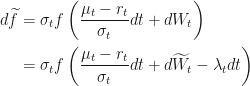
In the final step, we take Girsanov’s Theorem results:

$\displaystyle dW_t = d\widetilde{W}_t - \lambda_t dt$

and substitute it in to the original stochastic differential equation:

$\displaystyle dS_t = \mu_t S_t dt + \sigma_t S_t dW_t$

to get:

$\begin{aligned}dS_t &= \mu_t S_t dt + \sigma_t S_t dW_t \\ &= \mu_t S_t dt + \sigma_t S_t \left( d\widetilde{W}_t - \lambda_t dt \right) \\ &= \left( \mu_t S_t + \sigma_t S_t \lambda_t \right)dt + \sigma_t S_t d\widetilde{W}_t \\ &= S_t \left( \mu_t + \sigma_t \left( \frac{\mu_t - r_t}{\sigma_t}\right) \right)dt + \sigma_t S_t d\widetilde{W}_t \\ &= S_t \left( \mu_t + \left(\mu_t - r_t \right)\right)dt + \sigma_t S_t d\widetilde{W}_t \\ &= r_t S_tdt + \sigma_t S_t d\widetilde{W}_t\end{aligned}$

…and we are done!

We have successfully mixed the risky asset $dS_t = \mu_t S_t dt + \sigma_t S_t dW_t$ , with drift $\mu_t$ , with the risk-free asset $dB_t = r_t B_t dt$ , with risk-free interest rate $r_t$ , to produce a new risky asset $dS_t = r_t S_tdt + \sigma_t S_t d\widetilde{W}_t$ where the drift has been replaced by the risk-free interest rate.

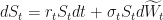
Under the risk-neutral probability measure $\mathbb{Q}$ , with Wiener process $\widetilde{W}_t$ , the drift of the risky asset $\mu_t$ becomes the risk-free interest rate $r_t$ .

Conclusion

In this blog, we considered a market consisting of just one risky asset and one risk-free asset. We assumed that the price dynamics of these two assets were driven by stochastic differential equations: the risky one by a Wiener process, and the risk-free one by a deterministic ordinary differential equation.

We then formed a new stochastic differential equation by continuously discounting the risky one by the risk-free rate. This new process was not a martingale under the original measure, because when we used Ito’s lemma to find the price dynamics of the new process, we found that it had huge amounts of drift: this huge amount we called the market price of risk.

Then we implemented Girsanov’s theorem to find a new probability measure such that the discounted price process is a martingale.

And finally, we found an equivalent risky asset price process, under the new probability measure, that was indeed a martingale again under the new measure.

If the risky asset is, say, the price of stock, then what we have just shown is that the discounted stock price is a martingale under the risk-neutral measure.

This allowed us to find a probability measure and Wiener process such that the drift is replaced by the risk-free interest rate.

The Recipe

Define a risky stochastic process, $S_t$ .
Define a risk-free stochastic process, $B_t$ .
Form some function or composition of the two: $f$ .
Use Ito’s product, or quotient lemma to find $df$ .
Rearrange and factor stuff to get $dW_t$ by itself.
Note the coefficient of $dt$ as lambda: $\lambda$ .
Implement Girsanov’s theorem and insert $\lambda$ in to the equation for $Z$ . Get $\mathbb{Q}$ .
State the results of Girsanov’s theorem, get $d\widetilde{W}_t$ .
Differentiate w.r.t. $t$ and rearrange to find $dW_t$ in terms of $d\widetilde{W}_t$ .
Form a new stochastic process under $\mathbb{Q}$ , and show that it should be drifless.
Implement the Martingale Representation Theorem. State equation of $f$ in terms of $\varphi$ .
Substitute $d\widetilde{W}_t$ back in to the original risky stochastic differential equation $dS_t$ . Rearrange, cancel stuff, factor, and get final $\mathbb{Q}$ -martingale.

References

Itô, Kiyosi, “Stochastic Integral” Proc. Imperial Acad. Tokyo 20, 519-524, (1944)
http://mathmistakes.info/facts/CalculusFacts/learn/doi/doi.html

One thought on “A Recipe for Pricing”

my-financial-wealth.com says:

January 18, 2021 at 5:55 PM

That’s interesting but too complex to understand 🙂

	Scarlett Tavores on The Hadamard Transform
	eo on Probability Distributions in…
	benjaminwhiteside on Options Hide in Taylor Se…
	Martin on Options Hide in Taylor Se…
	Veli on What is IRRBB?

From First Principles

Mathematics Without Hand Waving

A Recipe for Pricing

Introduction

The Black-Scholes Pricing Framework

What else do we need to assume?

Continuous discounting and the exponential

Practical Itô’s Lemma

1st Part

2nd Part

3rd Part

4th Part

Combining Parts for Ito’s Lemma

Rearrange to get dW Alone

Using Girsanov’s Theorem

Finding Lambda

The Martingale Representation Theorem

Final Step

Conclusion

The Recipe

References

One thought on “A Recipe for Pricing”

Leave a Reply Cancel reply

Introduction

The Black-Scholes Pricing Framework

What else do we need to assume?

Continuous discounting and the exponential

Practical Itô’s Lemma

1st Part

2nd Part

3rd Part

4th Part

Combining Parts for Ito’s Lemma

Rearrange to get dW Alone

Using Girsanov’s Theorem

Finding Lambda

The Martingale Representation Theorem

Final Step

Conclusion

The Recipe

References

Share this:

Like this:

One thought on “A Recipe for Pricing”

Leave a Reply Cancel reply