
Ever wondered what is so special about applying the Hadamard gate 
But how does this actually happen?
And more importantly: how was this discovered?
Like most exercises in quantum information theory you can either work forward or backward. Working forward through a problem is nice as it allows you to follow logical steps that lead from one proposition to the next. But often this hides the true motivation, and the result, which is usually remarkable, just happens to appear out of thin air.
As a researcher in this field, I find that working forward through a problem is not as useful as working backward through a problem. In this article we are also going to work backward through this problem because it is very easy to describe up front what we want.
We Want Entangled Qubits
It’s clear we want entangled qubits. One definition of an entangled system of qubits is that the state which describes the system cannot be factored as a product of states. But this definition is not very useful to us. Another definition is of the measurement of entangled qubits: that they are maximally correlated.
This is the definition we will use.
Two qubits are entangled when they are maximally correlated.
And this means that when we measure qubit one to be, say, 0 then qubit two is also 0. When we measure qubit one to be 1 then the second qubit is also 1, no matter what – they are maximally correlated. Even though a sequence of measurements may produce a random list of 0’s and 1’s, both lists from each qubit will be in the same order.
Only 4 Combinations to Think About
OK, so we want maximally correlated qubits. Let’s think about this in terms of two qubits, which we will label 


With just 2 qubits like this there are only 4 combinations possible:

and only two of these are correlated:

So, somehow, we must get rid of the states 

Writing Out States In Full
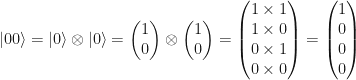
To give us an idea of where to go next, let us write out these quantum states in full.
The 

and the 

This is because the composite state 

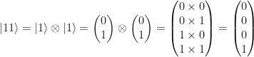
and so the full calculation of their tensor product is
and a similar calculation for the other correlated state:
It is very easy to see what happens when we add these two states together:

And now, what if we multiply this by 
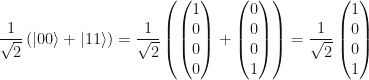
Why have I done this?
Well, because the state 
This is of no use to us because this is just a label we give to something we already know is maximally correlated, and hence entangled. But we do know how to get Bell states from other states.
This means that once we do a bunch of stuff (which we don’t know how to do yet!) and arrive at this Bell state, then we know immediately that the two qubits are maximally correlated.
So how do we get a Bell state?
Creating Bell States
There are many ways to create Bell states using quantum logic gates. But let’s say that we are researching this for the very first time and we don’t know any of these methods and we have to do it ourselves.
We know where we are starting from, because that is a register of two qubits 
and we know that we are only able to get there using quantum mechanics. This means we are only allowed to use unitary (density) matrices denoted by 

Therefore our problem becomes a matrix multiplication problem: Find a
There are so Many Unitaries!
The above system of linear equations must hold for every combination of qubit state placed in the 


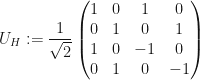
We can solve this equation using methods from linear algebra. This is too verbose for this blog, you can use your favourite mathematical software to solve it. But there does exist a
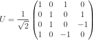
Before we check where this beast came from, let’s check that it works.
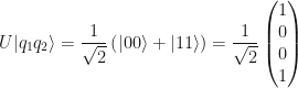
Checking the 00 State
Let’s begin by substituting all the necessary ingredients:
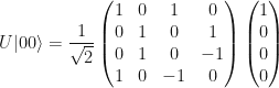
This calculation is very simple because of all the zeroes in the 


Those qubits are maximally correlated and we have successfully killed off the unwanted states.
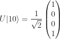
Checking the 10 State
What about the state

Success again! The only states left after this matrix multiplication by
Checking the 01 State
Let’s keep going! What about the state 
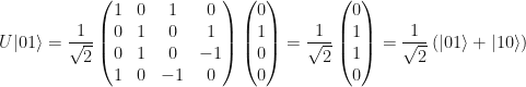
Whoa! Wait a minute.
That is NOT a correlated state there! What happened?
Well, technically they are maximally correlated…they’re just anti-correlated! Whenever the first qubit is a 1 the second is a 0, and vice versa. So technically, this is still something we desire! We just didn’t realise it. This is also a Bell state.
A Quick Note on the Basis
Interestingly, if we were calculating all of this stuff in the 

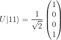
Checking the 11 State
OK, let’s keep going. What about the state
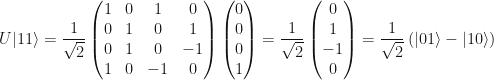
and again, this is anti-correlated and the 4th Bell state.
Deconstructing the Unitary
OK, so we successfully found a unitary matrix
that when applied to every single combination of input qubit states 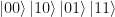
The question is now: How do we implement the unitary
Well, straight up, no – it’s not possible.
The trick is to note that 
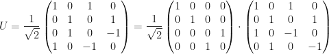
where

What is so special about this factorisation?
Well, both of these smaller matrices are both unitary as well, but they are also irreducible – they can’t be factored in to smaller unitaries. This means that they are implementable as quantum logic gates on a circuit.
In fact, these two matrices are already well-known as the CNOT gate 

Summary
So now we know that we can run any register of 2 qubits (no matter what state) through a Hadamard gate and then a CNOT gate will always result in a maximally correlated (or anti-correlated) pair of qubits.
By starting with what we wanted, we worked backward and expanded all the quantum states as vectors, solved a system of linear equations subject to the some constraints about unitary-ness, then factored that unitary matrix and found that the factors are the Hadamard and the CNOT gate.
We proved that this worked by working through the matrix multiplications of every single possible arrangement; and proved to ourselves that no matter which combination we put in to the Hadamard and CNOT gate arrangement we always ended up with what we wanted.
Doesn’t the CNOT Constitute a Measurement?
It make look like the CNOT gate must actually measure the first qubit to determine what to change the second gate to (or leave it). You might think therefore that the CNOT gate collapses the wavefunction or something like that – you know, like what a measurement does.
The CNOT gate never physically returns a result. It does not output a number or provide some status of the state of the system. Instead, it modifies the underlying probability distribution in a non-collapsing way. Very similar to quantum oracles, which act in the same way.
After a CNOT gate, the control qubit is kept while the target now holds the logical XOR of control-and-target so that

As you can see, this is difficult to do in practice as coherence must be ensured for as long as possible.
An example of a matrix which is not reversible and not unitary and which does collapse wavefunctions is the measurement matrix. An example of one acting on one qubit looks like this:
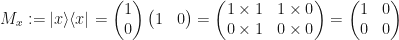
Very different kind of matrix when compared to the CNOT matrix.

beautiful definition/description. Never heard this backward way of explanation ever before. Just amazing. Please tell me you are a great professor in some great university. btw, there is a typo. checking the |10> section, you write U|01> – should be U|10>
Thanks for sharing such a useful insight.