Understanding Qubit Notation

Qubit notation can be pretty tricky to pick up, but it is extremely useful once you understand it.

Here is the mathematical representation of a bit:

$|\psi\rangle = \alpha|0\rangle + \beta|1\rangle$

Let’s deconstruct this.

Since a bit is a two-state system it can either ever be a $|0\rangle$ or a $|1\rangle$ . The numbers $\alpha,\,\beta$ represent the probability that the bit is measured in the $|0\rangle$ or the $|1\rangle$ state. The symbol $|\psi\rangle$ is the generic term for a bit, which could be in either state.

When we measure a bit it will either be in the $|0\rangle$ state or the $|1\rangle$ state – like an on/off switch (which is also a two-state system!) that when measured will be in either the Off state or the On state.

A bit, however, can never be in both states at the same time – this simply doesn’t make sense logically (and, I guess physically). An On/Off switch is only ever turned On or Off. Thus, we have a few restrictions on probabilities $(\alpha,\beta)$ . In particular, they can only ever take values 0 or 1 (representing 0% and 100%). Furthermore, whenever $\alpha = 1$ (which is when the bit is measured to be in $|0\rangle$ state) $\beta$ must equal 0, and vice versa.

A qubit, on the other hand, has exactly the same mathematical representation, but the constraints on the probabilities are lifted! They can now take on any value between 0% and 100%, so long as the following condition is satisfied:

$\displaystyle|\alpha|^2 + |\beta|^2 = 1$

So, for a bit, we could have:

$\displaystyle |\psi\rangle = 1|0\rangle + 0|1\rangle = |0\rangle$

But for a qubit, we could have:

$\displaystyle |\psi\rangle = \frac{1}{\sqrt{2}}|0\rangle + \frac{1}{\sqrt{2}}|1\rangle$

which works because it satsifies the constraint:

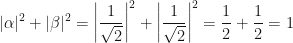
$\displaystyle |\alpha|^2 + |\beta|^2 = \left|\frac{1}{\sqrt{2}}\right|^2+\left|\frac{1}{\sqrt{2}}\right|^2=\frac{1}{2}+\frac{1}{2}=1$

Therefore,

$|\psi\rangle = \alpha|0\rangle + \beta|1\rangle$

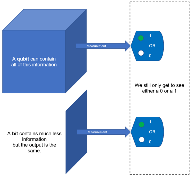
is a perfectly good representation of either a bit or a qubit, just with different restrictions on what the $\alpha$ and the $\beta$ parameters can and cannot do.

Figure 1 – Graphical representation of the extra pockets that qubits have. These can hold more information, but also require more physical degrees of freedom. However, upon measurement, both qubit and classical bit still only return a single bit of information!

Quantum Superposition

There is another name, a purely mathematical one, which describes a quantity which can be representated as $|\psi\rangle = \alpha |0\rangle + \beta |1\rangle$ – a linear combination. Thus, the quantity $|\psi\rangle$ , a qubit state, can always be written as a linear combination of its two measureable states. A classical bit cannot be written as a general linear combination because, as highlighted above, either one of $\alpha$ or $\beta$ must always be zero.

The terms superposition and linear combination are used almost synonymously when it comes to qubits. However, the term superposition should be reserved for a particular linear combination: the one where $\alpha$ and $\beta$ are both equal to $\frac{1}{\sqrt{2}}$ .

Now, why is that?

Well, as we shall see, with coefficients $\alpha, \beta = \frac{1}{\sqrt{2}}$ , the probability (which is the norm-squared of these numbers) turns out to equal exactly $\frac{1}{2}$ , which is 50%. So such a linear combination represents the possibility of measuring either the 0 state, or the 1 state, 50% of the time.

Keep in mind that this is not something which can be achieved with a classical bit.

We are about to see why this is so important!

The Hadamard Gate

Any qubit state $|\psi\rangle$ can be put in to such a superposition by applying the so-called Hadamard Gate. The Hadamard Gate is a square matrix that looks like this:

$\displaystyle H = \frac{1}{\sqrt{2}}\begin{bmatrix}1 & 1 \\ 1 & -1\end{bmatrix}$

and we have already seen it’s truth table in a previous blog, which also goes to show just how interesting this gate is, and how we just don’t have anything like it classically.

Let’s see what happens when we apply this gate to the $|0\rangle$ state:

$\displaystyle H|0\rangle = \frac{1}{\sqrt{2}}\begin{pmatrix}1 & 1 \\ 1 & -1\end{pmatrix}\begin{pmatrix}1 \\ 0\end{pmatrix} = \frac{1}{\sqrt{2}}\begin{pmatrix}1 \\ 1\end{pmatrix} = \frac{1}{\sqrt{2}}\begin{pmatrix}1 \\ 0\end{pmatrix} + \frac{1}{\sqrt{2}}\begin{pmatrix}0 \\ 1\end{pmatrix}$

$\displaystyle = \frac{1}{\sqrt{2}}|0\rangle + \frac{1}{\sqrt{2}}|1\rangle = \frac{|0\rangle + |1\rangle}{\sqrt{2}} =: |+\rangle$

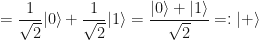
A similar calculation on the $|1\rangle$ states shows:

$\displaystyle H|1\rangle = \frac{1}{\sqrt{2}}\begin{pmatrix}1 & 1 \\ 1 & -1\end{pmatrix}\begin{pmatrix}0 \\ 1\end{pmatrix} = \frac{1}{\sqrt{2}}|0\rangle - \frac{1}{\sqrt{2}}|1\rangle = \frac{|0\rangle - |1\rangle}{\sqrt{2}} =: |-\rangle$

We can actually construct the Hadamard Gate matrix using outer products (this method of constructing gate matrices was also discussed in my previous blog post here):

$\displaystyle |+\rangle\langle 0| + |-\rangle\langle 1| = \frac{1}{\sqrt{2}}\begin{pmatrix}1 \\ 1\end{pmatrix}\begin{pmatrix}1 & 0\end{pmatrix}+\frac{1}{\sqrt{2}}\begin{pmatrix}1 \\ -1\end{pmatrix}\begin{pmatrix}0 & 1\end{pmatrix}=\frac{1}{\sqrt{2}}\begin{pmatrix}1 & 1 \\ 1 & -1\end{pmatrix}=H$

which is cool, and shows an alternative methods for coming up with the matrix itself, although guessing the exact combination for the outer product is not generally intuitive.

The Inner Product

The Inner Product (as opposed to the matrix-generating outer product discussed above) measures the angle between two vectors. It is a machine for combining two things and producing a real number. Symbolically, such a machine is written like this:

$\displaystyle \langle\cdot|\cdot\rangle\,:\,V\times V\longrightarrow\mathbb{R}$

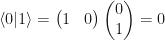
The two qubit states $|0\rangle$ and $|1\rangle$ can also have an angle-analogue between them. To compute them, we simply calculate their inner products:

$\displaystyle \langle 0|1 \rangle = \begin{pmatrix}1 & 0\end{pmatrix}\begin{pmatrix}0 \\ 1\end{pmatrix}=0$

Since this equals zero the two qubit states must be orthogonal to each other.

A similar calculation shows that the two states $|+\rangle$ and $|-\rangle$ are also orthogonal to each other:

$\langle +|- \rangle = \begin{pmatrix}\frac{1}{\sqrt{2}} & \frac{1}{\sqrt{2}}\end{pmatrix}\begin{pmatrix}\frac{1}{\sqrt{2}} \\ \frac{1}{\sqrt{2}}\end{pmatrix} = \frac{1}{\sqrt{2}} - \frac{1}{\sqrt{2}} = 0$

And since their lengths are also 1 (as discussed earlier), we say that both of these form an orthonormal basis. Such things are extremely important for bridging the gap between pure mathematical analysis (which doesn’t use numbers, but uses symbols) and applied physics (which use numbers).

Thus any quantum state $|\psi\rangle$ can be expressed as a linear combination (or superposition) of either of these pairs of basis states:

where again $|\alpha_0|^2 + |\alpha_1|^2 = |\alpha_+|^2 + |\alpha_-|^2 = 1$ .

Quantum Entanglement

To understand entanglement we must first understand two (-or more) qubit systems. In general, we would have one qubit $|\psi_1\rangle$ and a second qubit $|\psi_2\rangle$ together. We would write this like so:

$\displaystyle |\psi_1\psi_2\rangle$

This might be called in some contexts a quantum register. An example of a two qubit system might be the explicit all-zeroes state: $|00\rangle$ indicating that both qubits are in the 0 state. This two-qubit state can always be expanded as:

For a two-qubit system there can only ever be four outcomes:

$\displaystyle \left\{ |00\rangle, |01\rangle, |10\rangle, |11\rangle \right\}$

Just two of these states are interesting. Can you guess which ones?

Consider these two states $\left\{ |00\rangle, |11\rangle \right\}$ . What are these two states?

Well, if you were to measure the first qubit in either of these states you would immediately know the state of the other!

For example, in $|00\rangle$ , the first qubit is in the 0 state, and the second is also in the 0 state. They match! They don’t so much equal one another as they are correlated with one another. Measurement of a 0 in one means the other must be a 0, and similarly for a 1.

These states $\frac{1}{\sqrt{2}}(|00\rangle+|11\rangle)$ , and equivalently $\frac{1}{\sqrt{2}}(|00\rangle-|11\rangle)$ , are so special and peculiar that they are given a special name: Bell states.

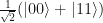
Bell states (and, in general, entangled states) are extremely powerful and could be said is the main reason why quantum computers are so powerful. Essentially, with a Bell state, you can make 1 measurement and obtain 2 bits of information, because once you measure the first qubit you gain knowledge of the second qubit because it’s 100% correlated.

Essentially, with a Bell state, you can make 1 measurement and obtain 2 bits of information!

Now, there isn’t anything particularly crazy going on here, after all, regular classical bits can also be in a similar situation. The problem is, for classical bits, there is just no way to get rid of the other two states $\left\{ |01\rangle, |10\rangle \right\}$ . They’re always there.

If we could remove those from existence then our entire universe would consist of the just two states $\left\{ |00\rangle, |11\rangle \right\}$ and knowing the first qubit would mean knowing the second. As it stands for regular bits, knowing the state of the first qubit gives you no knowledge of the second because the probability of it being 0 or 1 remains to be 50% each.

Is there a way that deletes those pesky $\left\{ |01\rangle, |10\rangle \right\}$ states and just leaves the interesting $\left\{ |00\rangle, |11\rangle \right\}$ states?

Yes there is! We can use destructive interference.

And it is only possible with qubits, you can’t do this with classical bits.

We do this with a combination of the Hadamard gate and the Controlled NOT gate. See my blog on how this is done here. But first, let us take a closer look in to the CNOT gate:

The CNOT Gate

So how does a CNOT Gate use the power of destructive interference to produce these highly correlated qubit states where essentially we are able to obtain 2 bits of information for 1?

As before, we begin with the truth table for a CNOT gate.

It’s easy to read this gate: If qubit A is a 0 then do nothing; else, if qubit A is 1 then switch B around.

The great thing about this is that it really makes it clear why the 0 state is so special and often employed along with the CNOT gate: If you CNOT anything with 0 you end up with anything … twice!

Don’t believe me? Well, what if I gave you 0? Then, from the above truth table, we have $\textup{CNOT}|00\rangle\mapsto|00\rangle$ . Cool, OK. So what if I now gave you 1? Then we have $\textup{CNOT}|10\rangle\mapsto|11\rangle$ .

See how both outputs are $|00\rangle$ and $|11\rangle$ ? We have essentially copied the input state on to the 0 state (in the computational basis). *whispers: we don’t get this if we use a different basis…

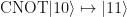
The CNOT gate essentially gives you the intriguing property that $\textup{CNOT}|x0\rangle\mapsto|xx\rangle$ ! I.e. the first state is copied on to the second, zero state.

OK, sounds like a legitimate logic gate. So why is this so special?

Let’s go a little further. Repeating what we did in a previous blog post, we can employ our general formula to create the matrix representation of this logic gate:

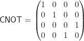
$\displaystyle\textsf{CNOT} = \begin{pmatrix}1 & 0 & 0 & 0 \\ 0 & 1 & 0 & 0 \\ 0 & 0 & 0 & 1 \\ 0 & 0 & 1 & 0\end{pmatrix}$

but this isn’t really helping us because we want to be able to see this gate as performing this map:

$\displaystyle \textsf{CNOT}|\psi_1 \psi_2\rangle \mapsto |\psi_1\rangle|\psi_1 \oplus \psi_2\rangle$

where $\oplus$ is addition modulo 2. But clearly, looking at not only the truth table above, but also thinking about the bottom-right corner of the CNOT matrix itself, the ordering of the last two qubit combinations (the $|10\rangle$ and the $|11\rangle$ combinations) are switched around.

This switching around of qubit combinations is not universal, however, as this operation does absolutely nothing to the first two combinations (the $|00\rangle$ and the $|01\rangle$ ones).

Specifically targeting the last two combinations is like a controlled NOT operation. It’s basically saying, if the first qubit state is a 1 then perform a NOT, i.e. if the second qubit state is a 0 then switch it to a 1, and vice versa.

This is why sometimes you see the CNOT gate written like this:

$\displaystyle \textsf{CNOT}|\psi_1, \psi_2\rangle = |\psi_1, \textsf{XOR}(\psi_1, \psi_2)\rangle$

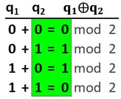
But now we have replace one question with another: why is the XOR gate like addition modulo 2?

XOR & Addition Modulo 2

This is an easy question to answer: so long as you are thinking in base 2.

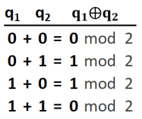
What is $1 + 1$ in base-2?

Well, in base-10 the answer is 2. But in base-2 there is no 2. 2 is 0. So $1+1 = 0 \bmod 2$ .

Continuing in this fashion we get:

So that’s addition modulo 2, what happens if we try replacing something with the NOT gate?

Easy.

Right, now going back to the list of 4 operations above, can we find the XOR pattern anywhere?

Yes we can:

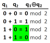
So we can just replace that with

We almost got there. Problem is, the NOT gate doesn’t cover the first two situations.

What can we do?

Well, we can try the exclusive-OR, or XOR gate. This will be controlled by the first qubit and the target qubit will be second qubit:

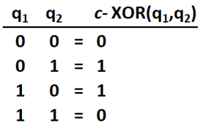
And now, can we find this pattern in modulo 2 arithmetic? Yes:

So we can just replace it:

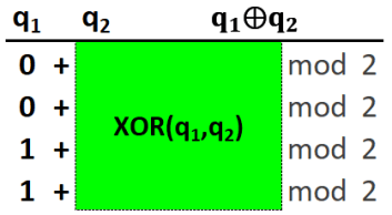
And now it should be clear that the addition modulo 2 of two qubits $q_1 \oplus q_2$ has the same truth table as a controlled-XOR, thus:

$\displaystyle |q_1\rangle\oplus|q_2\rangle = |\textsf{XOR}(q_1,q_2)\rangle$

Finally, since we already know that

$\displaystyle \textsf{CNOT}|q_1,q_2\rangle = |q_1,q_1\oplus q_2\rangle$

we must also have that

$\displaystyle \textsf{CNOT}|q_1,q_2\rangle = |q_1,\textsf{XOR}(q_1,q_2)\rangle$

where I have, admittedly, exchanged notation of qubits from $\psi_i$ to $q_i$ .

Summary

In this post we covered off qubit notation and explored a little bit of the CNOT gate and how it is used to entangle qubits – something which classical bits cannot do. The CNOT gate is an extremely important gate in quantum information theory, not just because it is one of the universal quantum gates but also because of how it is able to somehow react to the values of qubit states and alter underlying probability distributions without making a single, irreversible measurement. Yet, the CNOT gate has a classical, deterministic truth table! It is beyond my current understanding, however, how a CNOT gate is physically implemented as it appears to me to be quite a technical challenge due to its sensitivity to decoherence: you are essentially copying (without really copying) the state of the control qubit onto the state of the target qubit.

$\displaystyle \textsf{CNOT}|\psi_1 \psi_2\rangle \mapsto |\psi_1\rangle|\psi_1 \oplus \psi_2\rangle$

This act can be understood as performing a controlled XOR on the target qubit depending on the observed state of the first qubit – but this observation is done coherently.

Never-the-less, we can see that the CNOT gate has a matrix representation and it also can be represented as both an XOR gate and as addition modulo 2 (only because the computational basis is made up of 1’s and 0’s which just happen to be the only elements of base-2! Things get a tad more complicated in the +,- basis).

References

[1] Nielsen, N. & Chuang, I. L. – Quantum Computation and Quantum Information, Cambridge University Press, (2010).

	Scarlett Tavores on The Hadamard Transform
	eo on Probability Distributions in…
	benjaminwhiteside on Options Hide in Taylor Se…
	Martin on Options Hide in Taylor Se…
	Veli on What is IRRBB?

From First Principles

Mathematics Without Hand Waving

Understanding Qubit Notation

Quantum Superposition

The Hadamard Gate

The Inner Product

Quantum Entanglement

The CNOT Gate

XOR & Addition Modulo 2

Summary

References

Leave a Reply Cancel reply

Quantum Superposition

The Hadamard Gate

The Inner Product

Quantum Entanglement

The CNOT Gate

XOR & Addition Modulo 2

Summary

References

Share this:

Like this:

Leave a Reply Cancel reply