
You might have wondered (like myself) how a quantum algorithm actually achieves a result. After all, measurement of a bunch of qubits always reveals either a 1 or a 0, and the best quantum circuits that I’ve played with (as of September 2019) consist of a register of, at most, 14 qubits. So how does fourteen 1’s and 0’s and a bunch of logic gates actually form part of an algorithm?
If you have read the previous articles (here, here and here) then you will know that back in the 1920’s to the early 1950’s a computer was nothing but a sequence of switches whose sole purpose was to solve one particular mathematical problem. They weren’t like today’s multi-tasking computers. No, those old computers were one-trick ponies – and so are our early quantum computers.
Bits and qubits are both two-state systems. Bits interact with each other via the rules of Boolean logic while Qubits interact with each other via the rules of Quantum Mechanics.
When it comes to quantum algorithms we are no better off than where we were back in the 1950’s (reference, pg 39 of Computer Literature Bibliography here, CAMB49 – Some Routines Involving Large Integers (1949)); while in terms of hardware we are even further behind. For example, at the time of writing, the best available, public use quantum computer offers 72 qubits which puts us somewhere between the Model K from 1937 and the 400-relay Model I from Bell Labs in 1939. For a nice recount of Stibitz‘s early, low-count relay computers (and the error-correcting methods employed therein) see this article here from 1967.
List of Gate Model Quantum Processors
List current as of 10th October 2019.
- 2016 – IBM – Tenerife – 5qb
- 2016 – IBM – Yorktown – 5qb
- 2016 – IBM – Melbourne – 14qb
- 2017 – IBM – Seventeen – 17qb
- 2017 – Google – N/A – 20qb
- 2017 – Intel – N/A – 17qb
- 2017 – IBM – Tokyo – 20qb
- 2017 – Rigetti – Acorn – 19qb
- 2018 – Intel – Tangle Lake – 49qb
- 2018 – Google – Bristlecone – 72qb
- 2018 – IBM – Austin – 20qb
- 2018 – Rigetti – Aspen – 16qb
- 2019 – Google – Sycamore – 53qb
- 2019 – IBM – Prototype – 53qb
Types of Quantum Algorithms
For the past 20 years we have been building various quantum “computers” (or algorithms) to perform usually just one task, for example factoring a number in to primes.
For all the quantum algorithms that exist today (late 2019), which I think is upwards of 100, you can categorise them into the following main groups:
- Quantum Fourier Transform (QFT),
- Amplitude Amplification (AA),
- Quantum Walk (QW),
- Quantum Approximate Optimization Algorithm (QAOA), and
- Quantum Algorithms for Linear Systems (QALS).
There do exist other algortihms which don’t fit nicely in to these categories, for example quantum simulation and computing knot invariants, but we won’t really go in to these.
The five big categories of algorithms listed above contain the majority of research work, and each has their poster-child algorithm:
- Shor’s Algorithm (1994) – for finding the prime factors of an integer,
- Grover’s Algorithm (1996) – for searching data,
- Triangle Finding Algorithm (1999) – for finding triangles in graphs.
- QAOA Algorithm (2012/14) – self-titled.
- HHL Algorithm (2009) – for finding a scalar measurement on a linear system solution vector (not quite the actual solution!).
As you can see, most of these basic building blocks were proven well over a decade ago, and they are essentially analogous to the fundamental works of Boole, Shannon and Turing almost a century ago.
To understand these basic building blocks we must first understand how a binary relay circuit achieved its goals (for example, adding two numbers together – the so-called binary adder). Once we understand that, we can move on to a more abstract representation of the binary relay circuit and from there generalise it to what is going on in a quantum circuit.
The Binary Adder
This circuit, like most circuits we will be considering, performs one task: adding together two numbers. Further, the addition occurs in Base-2, but that’s OK, we will assume for now there is a conversion tool that first gets us in to Base-2 and then back to Base-10.
The Binary Adder circuit takes 2 inputs, sends those through an 


But how does an
The answer lies within their Truth Tables.
But first, let’s review binary arithmetic.
Binary Arithmetic
Suppose we want to calculate 


The problem with 


Thus, we have the following table:
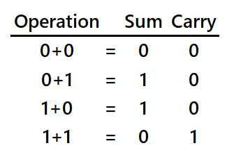
And from this basic understanding we can draw a skeleton circuit:
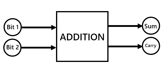
The goal now is to build the part of the circuit inside the black box so that the output bits are always what is seen on the right hand side of the table in Figure 1.
Consider now the
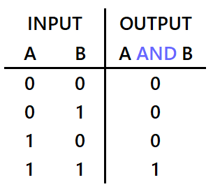
and the

Can you see that the

Well, that was easy!
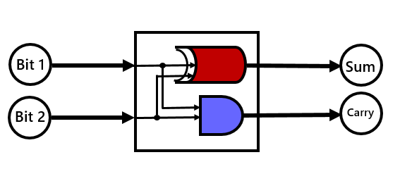
Let’s place the two gates in parallel. Let bit A equal 0 and bit B equal 0. First, send both 0’s through the
This whole circuit is called a binary Half-Adder.
Representing Gates as Matrices
Writing down truth tables gets very tedious very quickly for more than 1 bit systems. So in this section we will have a look at how to express binary truth tables as square matrices.
Why would we want to do that?
There are a few reasons. While being precisely equivalent to truth tables, the matrix representation also gives you nice, square matrices whose sizes can easily be increased to accommodate more and more bits. And the second benefit is that it a whole lot easier to quickly do the math when it comes to qubits! Square matrices also have the property that they could be unitary, but more on that later.
Take a look at the 
in matrix form this is simply:
But it is not as easy as simply putting the two columns of the truth table next to each other, there is a simple procedure for converting any truth table in to a matrix.
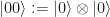
But first you have to assume that the True state 1 can be written as 

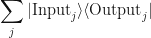
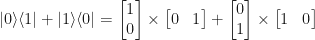
Once we make this convention, it is a simple matter to convert the truth table in to a matrix: we essentially follow the formula:
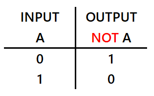
Worked Example: The NOT Gate
First, look at the truth table for the NOT gate and observe that the 0 goes to a 1 and the 1 goes to a 0. So we write:

Easy so far!
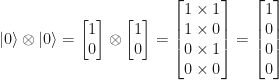
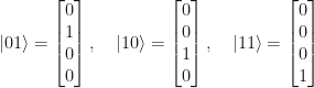
Now, write out the states in full vector form:
Even easier!
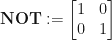
Now compute the matrix multiplications:

Add them all together:

Voila! A square matrix.
To check this works, let’s act on this matrix by the True state and see if it produces, through the magic of matrix multiplication, the False state (as it should since it is the NOT gate).

This exercise shows that truth tables can be represented as square matrices.
Two-bit Gates in Matrix Form
Let us now consider the two-bit CNOT truth table:

Unlike the other gates we have looked at, the CNOT gate produces two bits. What it says is: if the control bit (in our case A) is 0 then do nothing to the target bit (in our case B), else swap it around. Thus, if A=0 and B=0, then since A is 0 we do nothing to B, so we leave it as 0. However, if A=1 and B=0, then since A is 1 we flip B from 0 to 1.
Does the CNOT gate have a matrix representation?
Yes. And it looks like this:

Where did this funny looking matrix come from?
It is computed using the same formula from above:
Let’s see how it is done:
First, note that the truth table sends 00 to 00, 01 to 01, 10 to 11 and 11 to 10. We write this down as:

Easy so far!
But what is 
By definition it is nothing but
where the 
Similarly for the other 3 combinations:
Now, we can complete the formula:
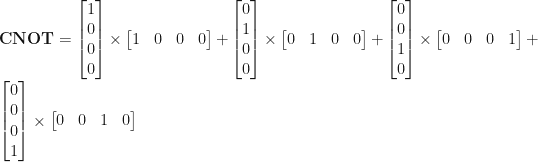
Which equals

As required.
Ready for Quantum Gates
So we have seen that we can perform mathematical operations (like addition) on binary numbers using nothing but logic gates. Those gates have matrix representations, which makes it easier to write down the input and output – simply by writing the input as a vector, matrix-multiplying it by the gate matrix, and observing the output vector. We have even seen how any truth table can be converted in to a square matrix with a little bit of effort.
Now we come to the point where we see why all that effort was needed.
Imagine if we had a truth table that looked like this:
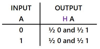
What is this gate doing?
This is a logic gate which changes its output each time it is used!
It says that if the input bit is a 0 then the output bit has an equal probability of being a 0 (as if no gate was there) and an equal probability of being a 1 (as if a NOT gate was there). Similarly if the input bit is a 1, then the output bit has an equal probability of being a 0 or a 1.
But this makes no sense.
How can a bit be both 0 and 1 at the same time?
So let’s assume for now that bits can magically have this property, what would this even allow us to do? Well, it would give us this new fancy looking gate. This gate takes an input bit and places it in to the unique output state that has equal probability of looking like no gate acted and like a NOT gate acted.
We call this gate the Hadamard gate.
A Hadamard gate is constantly changing the output as if it is not there 50% of the time and is a NOT gate the other 50% of the time.
That’s pretty cool.
If only bits could actually exist in such a state…
Or can they?
They can. Well, qubits can, ordinary classical bits cannot.
Probability
We have come to the point where Boolean algebra, logic and binary digits needs some probability injected in to it. The above Hadamard gate sends a binary bit in to some weird combination of both 0 and 1, with equal probability.
What is this probability?
This is the probability associated with observing the bit.
After the Hadamard gate acts on a bit (or we should say qubit from now on) the state of the qubit is in what is called a coherent superposition of its fundamental 0 and 1 states.
But it’s just a truth table!?
It is a truth table for a particular measurement of the gate output. The first time you run this circuit you might see the 0 go to a 0. The second time you could see the 0 go to a 1. Then 0 to a 0 again, then 0 to a 1, and so on. Do this one thousand times and you will likely get about five-hundred 0’s and five-hundred 1’s. It’s a form of an ever-changing logic gate – but what isn’t changing is the probability. It’s always 50% 0 and 50% 1.
So, a Hadamard gate is constantly changing the output as if it is not there 50% of the time and is a NOT gate the other 50% of the time. We call those two 50%’s the probability amplitudes for the two states.
A nice way to write this down is: regardless of the input value (0 or 1), let’s just call it 

This is called a superposition of states and is something that ordinary bits just cannot do; they can never be in this state because ordinary bits are always in one state or the other, even when you are not looking at them. Thus, a there is a deep, physical dependency on the existence of the quantum-like Hadamard gate and the quantum-ness inherit in a qubit.
Does the Hadamard gate have a matrix too?
Yes it does, but before we can show you we need to understand probability amplitudes a bit better, namely, why they are square roots. Otherwise you’ll have no idea where the little 
Summary
In this article we made the leap from relays to binary bits. Bits can be passed through logic gates that re-arrange the binary states of the bit; each logic gate has a truth table associated with. By considering first what it takes to add a binary number together, we can create the exact same behaviour of addition with an AND and an XOR gate arranged in parallel.
Then we generalised our truth tables to matrix representations and by doing this we could cut down the amount of computation we need to do by performing matrix multiplication. Further, matrices could handle larger truth tables with multiple input and output bits a lot better.
Finally, we introduced a funny looking truth table that keeps changing every time we look at it. From one observation to the next it acts either like a NOT gate or no gate at all.
In the next article, we will investigate further why this strange logic gate manifests quantum behaviour. We will look at probability amplitudes and explain the matrix representation of this gate. Finally, this will lead us to a better understanding of quantum logic gates as a whole – and we might even meet our first quantum calculator!
See Also
References
[1] Stibitz, G. R. & Loveday, E., The relay computers at Bell Labs, Datamation (1967).
