Transforming Stochastic Processes: Girsanov's Theorem in SageMath

Introduction

In the previous blogs we taught SageMath how to represent stochastic differential equations (as a data class), apply Ito’s lemma (as part of our Ito package), derive infinitesimal generators, and connect those generators to the Kolmogorov equations. We also introduced exponential martingales in the previous blog, and now, in this blog, that implementation will become useful because Girsanov’s theorem tells us how to change probability measure by reweighting paths, and in doing so, how to rewrite the drift of an SDE while leaving its diffusion term unchanged.

Motivation

Up to this point, our SageMath/Ito framework has been working quietly under the assumption that there is only one probability measure. This was totally fine while we were focusing on:

deriving SDE dynamics using Ito’s lemma,
constructing infinitesimal generators, and
linking those generators to the Kolmogorov equations.

But the moment we try to connect this machinery to financial modelling, the assumption of a single probability measure breaks down!

In practice, we almost never work with a single probability measure!

We typically start with a physical model of the world, these are events which we can actually, physically, observe. This is the physical measure or the real-world measure, and it’s usually denoted with $\mathbb{P}$ .

However, pricing financial derivatives requires working under the risk-neutral measure, denoted $\mathbb{Q}$ , which is a special probability measure than makes discounted asset prices martingales.

So, we must systematically transform an SDE from one measure to another, whilst keeping the underlying stochastic structure in tact.

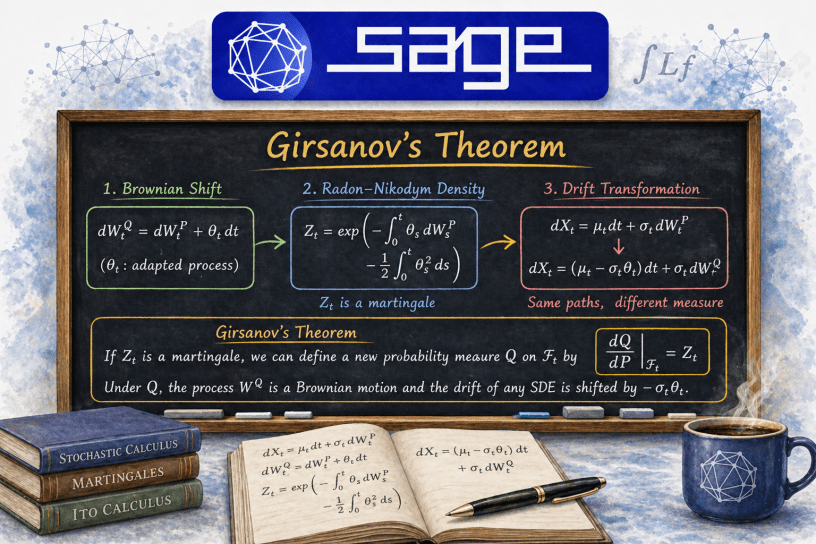
Girsanov’s theorem to the rescue!

This theorem tells us that we can reweight the paths of the stochastic process so that the Brownian motion absorbs a drift adjustment, and the resulting dynamics are expressed under a new probability measure in which suitable processes (functionals like discounted asset prices) become martingales.

The exponential martingale now becomes the central object for this blog. It previously appeared as a formal construction, but now it will take on a concrete role: it will be the object which links $\mathbb{P}$ with $\mathbb{Q}$ . It will be the thing which does the reweighting. It will be the Radon-Nikodym derivative.

Our new module girsanov.py will implement all of this directly at the SDE class object level. Thus, given

an SDE1D object,
a drift shift $\theta$ , and a
source and target probability measure

it will construct:

a BrownianShift1D object, which encodes the data for the change of measure $dW_t^{\mathbb{Q}} = dW_t^{\mathbb{P}} + \theta_t dt$ ,
a method that calculates the transformed_drift() which computes $\mu_{\mathbb{Q}} = \mu_{\mathbb{P}} - \sigma\theta$ ,
the new, transformed 1-dimensional SDE under the target measure, and
the associated density process $\Lambda$ .

Implementation

To recap, so far we have built a lot of things, such as

Ito algebra class, which gives a symbolic differential layer,
ito_lemma method, which is our transformation engine,
lamperti_transform gives us diffusion normalisation,
generator plus kolmogorov gives us partial differential equations, and
SDE1D is the user-facing abstraction for 1-dimensional stochastic differential equations.

This gives us a pipeline:

$\displaystyle \text{SDE} \rightarrow \text{Ito} \rightarrow \text{Generator} \rightarrow \text{PDE} \rightarrow \text{Transformations}$

This is precisely what we need before we can even start thinking about Girsanov’s theorem. But we are missing one more ingredient!

Measure awareness.

Right now, everything lives in a single, unnamed probability measure, so we need to introduce the Python equivalent of the following statement: “This SDE is defined under the measure P, and we want to move to Q“.

So far, our Brownian motion and our probability measure is implicitly P and the drift is just a drift. Now we need to be explicit!

We are going to build the following simple data class inside the Sde package because its purpose is to transform an existing, symbolically defined, stochastic differential equation from one probability measure to another.

This module is built around three main class objects:

BrownianShift1D
RadonNikodymDensity1D
GirsanovTransform1D

The Brownian Shift Class

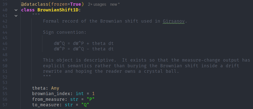
The first object, BrownianShift1D, records the formal Brownian motion shift used in the measure change. With the sign convention used:

$\displaystyle dW_t^{\mathbb{Q}} = dW_t^{\mathbb{P}} + \theta_t dt$

It does not try to simulate Brownian motion nor perform any sort of stochastic integration. Instead, it is a data class, it simply records the semantic meaning of the measure change and provides the text and LaTeX descriptions of the Brownian shift.

This is useful because otherwise the drift rewrite would happen silently, and I want to see it! The class stores this drift shift in the parameter $\theta$ , and it also exposes a Jupyter notebook output so we can display it in LaTeX.

Code

@dataclass(frozen=True)
class BrownianShift1D:
    """
        Formal record of the Brownian shift used in Girsanov.
        Sign convention:
            dW^Q = dW^P + theta dt
            dW^P = dW^Q - theta dt
        This object is descriptive.  It exists so that the measure-change output has
        explicit semantics rather than burying the Brownian shift inside a drift
        rewrite and hoping the reader owns a crystal ball.
        """
    theta: Any
    brownian_index: int = 1
    from_measure: str = "P"
    to_measure: str = "Q"
    def differential_under_new_measure(self) -> str:
        """Return the formal differential relation dW^Q = dW^P + theta dt."""
        i = self.brownian_index
        return f"dW{i}^{self.to_measure} = dW{i}^{self.from_measure} + ({self.theta}) dt"
    def old_brownian_in_terms_of_new(self) -> str:
        """Return the formal inverse relation dW^P = dW^Q - theta dt."""
        i = self.brownian_index
        return f"dW{i}^{self.from_measure} = dW{i}^{self.to_measure} - ({self.theta}) dt"
    def to_latex(self) -> str:
        theta_ltx = latex(self.theta)
        i = self.brownian_index
        return (
            rf"dW^{{{self.to_measure}}}_{{{i}}}"
            rf"= dW^{{{self.from_measure}}}_{{{i}}} + {theta_ltx}\,dt"
        )
    def describe(self) -> Dict[str, Any]:
        return {
            "type": "BrownianShift1D",
            "from_measure": self.from_measure,
            "to_measure": self.to_measure,
            "brownian_index": self.brownian_index,
            "theta": self.theta,
            "relation": self.differential_under_new_measure(),
            "inverse_relation": self.old_brownian_in_terms_of_new(),
            "latex": self.to_latex(),
        }

The Radon-Nikodym Density Class

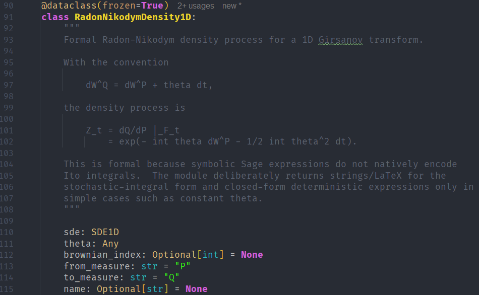
The next object, RadonNikodymDensity1D, represents the density process associated with the measure change.

Under our convention,

$\displaystyle dW_t^{\mathbb{Q}} = dW_t^{\mathbb{P}} + \theta_t dt$

the Radon-Nikodym density is represented formally, and symbolically using SageMath, as

$\displaystyle Z_t = \exp\left(-\int_0^t \theta_s dW_s^{\mathbb{P}} - \frac{1}{2}\int_0^t \theta_s^2 ds\right)$

which we already know works because it is the ExponentialMartingale1D class object from the previous blog!

Again, this object is deliberately formal, because SageMath symbolic expressions do not natively encode Ito integrals, and it also provides string and LaTeX representations of the stochastic integral form.

Code

@dataclass(frozen=True)
class RadonNikodymDensity1D:
    """
    Formal Radon-Nikodym density process for a 1D Girsanov transform.
    With the convention
        dW^Q = dW^P + theta dt,
    the density process is
        Z_t = dQ/dP |_F_t
            = exp(- int theta dW^P - 1/2 int theta^2 dt).
    This is formal because symbolic Sage expressions do not natively encode
    Ito integrals.  The module deliberately returns strings/LaTeX for the
    stochastic-integral form and closed-form deterministic expressions only in
    simple cases such as constant theta.
    """
    sde: SDE1D
    theta: Any
    brownian_index: Optional[int] = None
    from_measure: str = "P"
    to_measure: str = "Q"
    name: Optional[str] = None
    def __post_init__(self):
        if self.brownian_index is None:
            object.__setattr__(self, "brownian_index", self.sde.dw_index)
    def exponential_martingale(self, simplify_result: bool = True) -> ExponentialMartingale1D:
        """
        Returns the matching ExponentialMartingale1D object already used by the
        existing Ito layer.
        """
        return ExponentialMartingale1D.from_theta(
            self.sde,
            theta=self.theta,
            brownian_index=self.brownian_index,
            name=self.name,
            simplify_result=simplify_result,
        )
    def ito_integral_str(self) -> str:
        return f"int_0^{self.sde.t} ({self.theta}) dW{self.brownian_index}^{self.from_measure}"
    def dt_integral_str(self) -> str:
        return f"int_0^{self.sde.t} ({self.theta})**2 ds"
    def formal(self) -> str:
        return f"exp(-{self.ito_integral_str()} - 1/2*{self.dt_integral_str()})"
    def to_latex(self) -> str:
        theta_ltx = latex(self.theta)
        t_ltx = latex(self.sde.t)
        i = self.brownian_index
        return (
            r"\exp\!\left("
            + rf"-\int_0^{{{t_ltx}}} {theta_ltx}\,dW^{{{self.from_measure}}}_{{{i}}}"
            + rf"-\frac{{1}}{{2}}\int_0^{{{t_ltx}}} \left({theta_ltx}\right)^2\,ds"
            + r"\right)"
        )
    def constant_theta_closed_form(self, w: Any, simplify_result: bool = True) -> Any:
        """
        Closed form when theta is deterministic/constant with respect to the
        Brownian variable w:
            Z(t, w) = exp(-theta*w - 1/2 theta**2*t)
        The caller supplies w, usually a symbolic variable representing W_t.
        """
        theta = self.theta
        expr = exp(-theta * w - SR(1) / SR(2) * theta**2 * self.sde.t)
        return _simplify(expr, simplify_result=simplify_result)
    def verify_constant_theta_martingale_pde(self, w: Any, simplify_result: bool = True) -> Dict[str, Any]:
        """
        Verify the backward heat equation for constant theta:
            Z_t + 1/2 Z_ww = 0.
        This mirrors the verification method in ExponentialMartingale1D, but is
        included here so the Girsanov density can be tested directly.
        """
        Z = self.constant_theta_closed_form(w, simplify_result=False)
        Z_t = diff(Z, self.sde.t)
        Z_ww = diff(Z, w, 2)
        residual = Z_t + SR(1) / SR(2) * Z_ww
        return {
            "Z": _simplify(Z, simplify_result),
            "Z_t": _simplify(Z_t, simplify_result),
            "Z_ww": _simplify(Z_ww, simplify_result),
            "residual": _simplify(residual, simplify_result),
        }
    def describe(self) -> Dict[str, Any]:
        return {
            "type": "RadonNikodymDensity1D",
            "name": self.name,
            "from_measure": self.from_measure,
            "to_measure": self.to_measure,
            "brownian_index": self.brownian_index,
            "theta": self.theta,
            "formal": self.formal(),
            "latex": self.to_latex(),
        }

The Girsanov Transform Class

The central object in this implementation is the GirsanovTransform1D class object. This class takes in:

an existing SDE1D class object,
a drift shift $\theta$ ,
labels for the original and target probability measures

and its job is to package the data required for the Girsanov transformation into one data class.

This is what it does symbolically, step-by-step.

Start with the original SDE:

$\displaystyle dX_t = \mu dt + \sigma dW_t^{\mathbb{P}}$

symbolically infer the (1-dimensional) Brownian shift

$\displaystyle dW_t^{\mathbb{Q}} = dW_t^{\mathbb{P}} + \theta_t dt$

calculate the transformed SDE:

$\displaystyle dX_t = (\mu - \sigma\theta)dt + \sigma dW_t^{\mathbb{Q}}$

which is implemented directly in transformed_drift(), which computes:

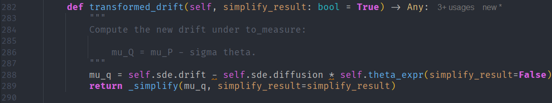
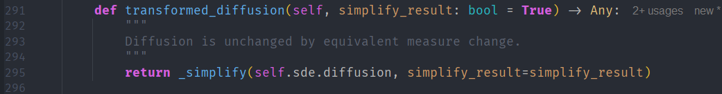
Code snippet displaying a Python function definition for 'transformed_drift', including comments and calculations related to drift and diffusion. — **Fig 3** – The `transformed_drift()` class method of the `GirsanovTransform` class object in PyCharm.

while the transformed_diffusion() method leaves the diffusion coefficient unchanged:

Python code snippet defining a function named 'transformed_diffusion', which describes diffusion in relation to equivalent measure change. — **Fig 4** – The `transformed_diffusion()` class method of the `GirsanovTransform` class object in PyCharm.

The transformed_sde() method then constructs a new SDE1D object using the transformed drift and the original diffusion:

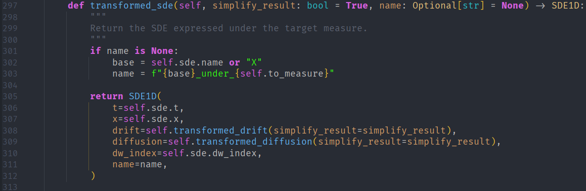
Code snippet showing a Python function definition for 'transformed_sde' with parameters for simplifying results and naming, returning an instance of SDE1D. — **Fig 5** – The `transformed_sde()` class method of the `GirsanovTransform` class object in PyCharm.

The class also exposes helper methods for applying the new-measure generator and Ito operator. This is important because the transformed SDE is not just a display object. Once the measure change has been applied, the resulting SDE can be passed back into the existing machinery for generators, Kolmogorov equations, and PDE checks. In other words, the Girsanov transform becomes another step in the symbolic SDE pipeline rather than a dead-end calculation.

Helper Methods

Finally, the module provides convenience constructors. The most useful one is theta_for_target_drift(). Instead of manually specifying $\theta$ , we can specify the desired target drift and solve

$\displaystyle \mu_{\text{target}} = \mu_{\text{original}} - \sigma\theta$

Rearranging gives:

$\displaystyle \theta = \frac{\mu_{\text{original}} - \mu_{\text{target}}}{\sigma}$

which is exactly what we need for financial experiments such as transforming geometric Brownian motion from the physical drift $\mu S_t$ to a risk-neutral drift $r S_t$ . The wrapper gbm_risk_neutral_transform() specialises this pattern by setting the target drift to $rx$ , where $x$ is the state variable of the SDE.

Summary of the Girsanov Transform Class

The module has the structure:

BrownianShift1D: records how the Brownian motion changes,
RadonNikodymDensity1D: records the density process that reweights the paths,
GirsanovTransform1D: applies the induced drift change to the original SDE,
Helper functions: can solve for $\theta$ when the target drift is known.

Code

@dataclass(frozen=True)
class GirsanovTransform1D:
    """
    Symbolic 1D Girsanov transform for an SDE1D.
    Parameters
    ----------
    sde:
        Original SDE under from_measure.
    theta:
        Market price of risk / Brownian drift shift.  May be constant, a Sage
        expression in (t, x), or anything Sage can carry symbolically.
    from_measure:
        Original measure label, default "P".
    to_measure:
        New measure label, default "Q".
    name:
        Optional transform label.
    Mathematical convention
    -----------------------
    Given
        dX = mu dt + sigma dW^P,
    and
        dW^Q = dW^P + theta dt,
    the transformed Q-dynamics are
        dX = (mu - sigma theta) dt + sigma dW^Q.
    """
    sde: SDE1D
    theta: Any
    from_measure: str = "P"
    to_measure: str = "Q"
    name: Optional[str] = None
    def theta_expr(self, simplify_result: bool = True) -> Any:
        """Return theta, optionally simplified."""
        return _simplify(_coerce_symbolic(self.theta), simplify_result=simplify_result)
    def brownian_shift(self, simplify_result: bool = True) -> BrownianShift1D:
        """Return the formal Brownian shift object."""
        return BrownianShift1D(
            theta=self.theta_expr(simplify_result=simplify_result),
            brownian_index=self.sde.dw_index,
            from_measure=self.from_measure,
            to_measure=self.to_measure,
        )
    def density(self, simplify_result: bool = True) -> RadonNikodymDensity1D:
        """Return the formal Radon-Nikodym density process Z_t."""
        return RadonNikodymDensity1D(
            sde=self.sde,
            theta=self.theta_expr(simplify_result=simplify_result),
            brownian_index=self.sde.dw_index,
            from_measure=self.from_measure,
            to_measure=self.to_measure,
            name=self.name,
        )
    def exponential_martingale(self, simplify_result: bool = True) -> ExponentialMartingale1D:
        """Return the density process as the existing ExponentialMartingale1D."""
        return self.density(simplify_result=simplify_result).exponential_martingale(
            simplify_result=simplify_result
        )
    def original_drift(self) -> Any:
        return self.sde.drift
    def original_diffusion(self) -> Any:
        return self.sde.diffusion
    def transformed_drift(self, simplify_result: bool = True) -> Any:
        """
        Compute the new drift under to_measure:
            mu_Q = mu_P - sigma theta.
        """
        mu_q = self.sde.drift - self.sde.diffusion * self.theta_expr(simplify_result=False)
        return _simplify(mu_q, simplify_result=simplify_result)
    def transformed_diffusion(self, simplify_result: bool = True) -> Any:
        """
        Diffusion is unchanged by equivalent measure change.
        """
        return _simplify(self.sde.diffusion, simplify_result=simplify_result)
    def transformed_sde(self, simplify_result: bool = True, name: Optional[str] = None) -> SDE1D:
        """
        Return the SDE expressed under the target measure.
        """
        if name is None:
            base = self.sde.name or "X"
            name = f"{base}_under_{self.to_measure}"
        return SDE1D(
            t=self.sde.t,
            x=self.sde.x,
            drift=self.transformed_drift(simplify_result=simplify_result),
            diffusion=self.transformed_diffusion(simplify_result=simplify_result),
            dw_index=self.sde.dw_index,
            name=name,
        )
    def transformed_differential(self, simplify_result: bool = True) -> Ito:
        """Return dX under the target measure as an Ito object."""
        return self.transformed_sde(simplify_result=simplify_result).dX()
    def drift_change(self, simplify_result: bool = True) -> Any:
        """
        Return the drift adjustment applied to the original drift:
            mu_Q - mu_P = -sigma theta.
        """
        delta = -self.sde.diffusion * self.theta_expr(simplify_result=False)
        return _simplify(delta, simplify_result=simplify_result)
    def generator_under_new_measure(self, f: Any, simplify_result: bool = True) -> Any:
        """
        Apply the target-measure spatial generator to f:
            L_Q f = (mu - sigma theta) f_x + 1/2 sigma**2 f_xx.
        """
        return self.transformed_sde(simplify_result=simplify_result).generator(
            f,
            simplify_result=simplify_result,
        )
    def ito_operator_under_new_measure(self, f: Any, simplify_result: bool = True) -> Any:
        """
        Apply the target-measure Ito operator to f:
            (d/dt + L_Q) f.
        """
        return self.transformed_sde(simplify_result=simplify_result).ito_operator(
            f,
            simplify_result=simplify_result,
        )
    def verify_target_drift(self, target_drift: Any, simplify_result: bool = True) -> Dict[str, Any]:
        """
        Compare the transformed drift against a supplied target drift.
        Useful for examples such as GBM under P -> risk-neutral Q, where the
        target drift is r*S.
        """
        mu_q = self.transformed_drift(simplify_result=False)
        residual = mu_q - target_drift
        return {
            "target_drift": target_drift,
            "transformed_drift": _simplify(mu_q, simplify_result),
            "residual": _simplify(residual, simplify_result),
            "matches": _simplify(residual, simplify_result) == 0,
        }
    def describe(self, simplify_result: bool = True) -> Dict[str, Any]:
        """Return a structured summary of the transform."""
        transformed = self.transformed_sde(simplify_result=simplify_result)
        shift = self.brownian_shift(simplify_result=simplify_result)
        density = self.density(simplify_result=simplify_result)
        return {
            "type": "GirsanovTransform1D",
            "name": self.name,
            "from_measure": self.from_measure,
            "to_measure": self.to_measure,
            "original_sde": repr(self.sde),
            "theta": self.theta_expr(simplify_result=simplify_result),
            "brownian_shift": shift.describe(),
            "density": density.describe(),
            "original_drift": self.sde.drift,
            "drift_change": self.drift_change(simplify_result=simplify_result),
            "transformed_drift": transformed.drift,
            "transformed_diffusion": transformed.diffusion,
            "transformed_sde": repr(transformed),
        }
    def __repr__(self) -> str:
        label = f"{self.name}: " if self.name else ""
        return (
            f"{label}GirsanovTransform1D("
            f"{self.from_measure}->{self.to_measure}, "
            f"theta={self.theta})"
        )

Results

Geometric Brownian Motion

To illustrate the girsanov.py module in practice, let us consider our usual first test case of standard geometric Brownian motion (GBM), and this time we say that it is under the physical measure $\mathbb{P}$ :

$\displaystyle dS_t = \mu S_t dt + \sigma S_t dW_t^{\mathbb{P}}$

We require GBM under the risk-neutral measure $\mathbb{Q}$ , so:

$\displaystyle dS_t = r S_t dt + \sigma S_t dW_t^{\mathbb{Q}}$

The goal of this demo is to show how the GirsanovTransform1D object connects these two SDEs in a completely symbolic way.

Step 1: Constructing the Transform

Rather than manually specifying the drift shift $\theta$ , we use the in-built helper method to compute

$\displaystyle \theta = \frac{\mu - r}{\sigma}$

This is computed internally by theta_for_target_drift(sde, target_drift=r*S):

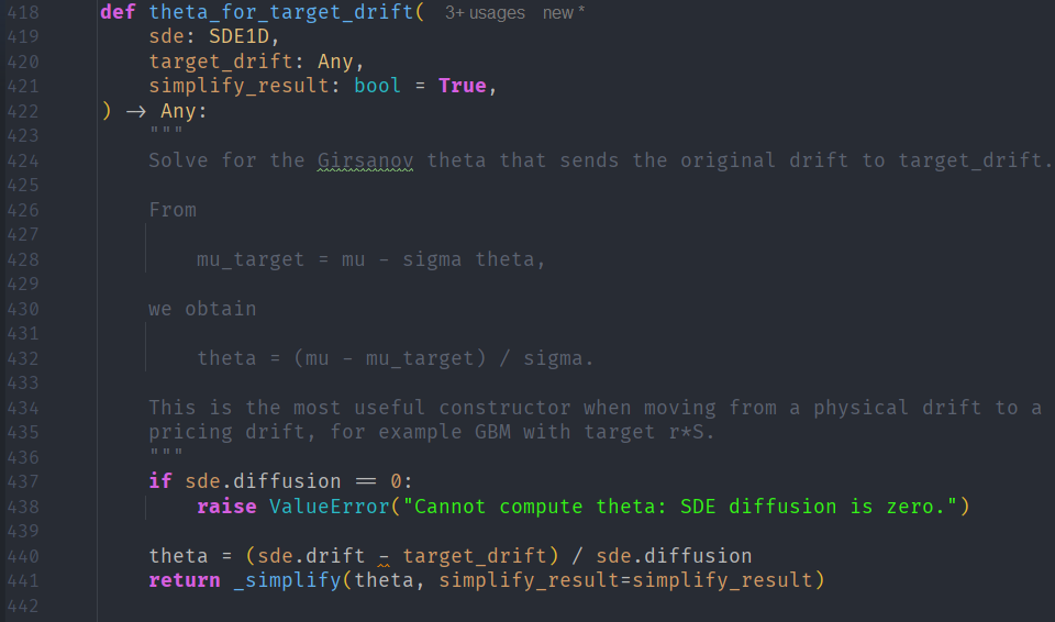
A code snippet in Python defining a function for calculating the Girsanov theta for target drift in stochastic differential equations (SDE). — **Fig 6** – The `GirsanovTransform` helper method `theta_for_target_drift()` in PyCharm.

which solves

$\displaystyle \mu_{\mathbb{Q}} = \mu_{\mathbb{P}} - \sigma\theta$

Already we see a subtle but important design choice: we specify the target behaviour, and let the framework infer the required measure change.

Step 2: The Brownian Shift

The Jupyter Notebook then displays

$\displaystyle dW_t^{\mathbb{Q}} = dW_t^{\mathbb{P}} + \frac{\mu - r}{\sigma}dt$

Mathematical equations related to financial modeling, including formulas for theta, original drift, drift adjustment, new drift under Q, unchanged diffusion, and Brownian shift. — **Fig 7** – The Brownian Shift displayed as LaTeX in Jupyter Notebook, all symbols derived automatically by SageMath and our Ito algebra class.

This tells us that:

we are not changing the paths themselves, and
we are reinterpreting the Brownian motion under a new measure.

This data object comes directly from BrownianShift1D, which is the data class we implemented to make this particular step explicit.

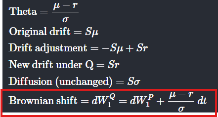
Step 3: Drift Transformation

The transformed drift is computed as:

$\displaystyle \mu_{\mathbb{Q}} = \mu_{\mathbb{P}} - \sigma\theta =: r$

The Jupyter Notebook output confirms:

we still have the original drift: $\mu S_t$ ,
we have the transformed drift: $r S_t$ , and
the diffusion is unchanged at: $\sigma S$ .

Step 4: The Density Process

We also get SageMath to output the Radon-Nikodym density:

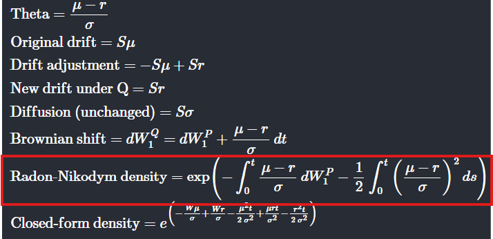
Mathematical equations related to stochastic processes and Radon-Nikodym density, including drift adjustments and closed-form density expressions. — **Fig 8** – The Radon-Nikodym density as output by SageMath with all symbols derived automatically by SageMath together with our Ito algebra class.

This is the Exponential Martingale from the previous blog, except now constructed symbolically from first principles, rendered in LaTeX in a Jupyter Notebook, and also (optionally) converted into a closed-form expression only when $\theta$ is constant.

This is the thing which actually reweights the Brownian paths!

So, for GBM, with constant $\theta$ , the density actually simplifies into:

$\displaystyle Z_t = \exp\left(-\theta W_t - \frac{1}{2}\theta^2 t\right)$

The demo code (not Jupyter Notebook) verifies this explicitly and even checks to see if it satisfies the backward heat equation:

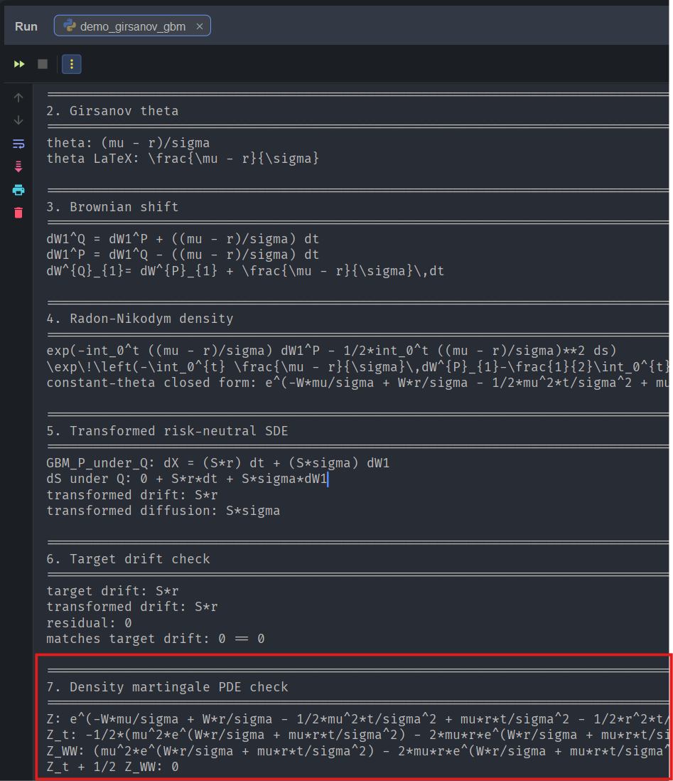
Screenshot of a code environment displaying mathematical concepts related to finance, including Girsanov's theorem, Brownian shift, Radon-Nikodym density, transformed risk-neutral SDE, and density martingale PDE check. — **Fig 9** – Console output of the `demo_girsanov_gbm.py` test showing, among other things, that the solution satisfies the backward heat equation. This proves that the density process that SageMath derived symbolically is not just formal, but behaves exactly like a martingale should.

Conclusion

This test has shown that we can:

symbolically define (1-dimensional) SDEs,
symbolically define measure changes, and
symbolically derive a density process associated with that measure change.

This is achieved, in a structured way, through the girsanov.py module; and it ties together several ideas from earlier posts. The exponential martingale is no longer a formal curiosity; it becomes the object that defines the change of measure. The generator and Kolmogorov machinery remain intact, but now operate under a transformed drift. The SDE itself becomes something that can be reinterpreted under different probabilistic worlds rather than a fixed object tied to a single measure.

The geometric Brownian motion example illustrates this clearly. Starting from physical dynamics, we use the framework to construct the risk-neutral measure, recover the correct drift, and explicitly represent the density process that links the two. More importantly, we can verify that this density behaves as expected, satisfying the martingale PDE in the constant- $\theta$ case.

Next Steps

The current implementation is intentionally focused on the one-dimensional case. The most immediate extension is to move to multi-dimensional SDEs, where the Brownian motion becomes vector-valued and the drift shift $\theta$ interacts with a covariance structure. This introduces additional complexity, but the underlying ideas remain the same.

Another natural direction is to tighten the connection with the Kolmogorov equations and the Feynman–Kac framework. Under a change of measure, the generator changes, and so do the associated PDEs. Making this transformation explicit would allow the framework to move seamlessly between SDE representations and pricing equations.

There is also scope to improve the symbolic handling of stochastic integrals. At present, the Radon–Nikodym density is represented formally, with closed-form expressions available only in simple cases such as constant $\theta$ . Extending this to richer classes of processes would make the framework more expressive and reduce the reliance on manual interpretation.

Finally, and perhaps most importantly, the framework can now be applied to more interesting models. Ornstein–Uhlenbeck processes, CIR dynamics, and other mean-reverting systems all involve non-trivial drift structures where measure changes are essential. Applying Girsanov in these settings will test the robustness of the implementation and expose any hidden assumptions that GBM politely ignored. We will cover these tests in the next blog.

References

SageMath home page
https://doc.sagemath.org/html/en/reference/calculus/index.html
Øksendal, B. (2003). Stochastic Differential Equations.
Karatzas & Shreve (1991). Brownian Motion and Stochastic Calculus.
https://en.wikipedia.org/wiki/Girsanov_theorem
https://en.wikipedia.org/wiki/Radon–Nikodym_theorem#Radon–Nikodym_derivative

	Muhammad Shumail on Hadamard & CNOT
	spiral on A Recipe for Pricing
	Deutsch-Jozsa Algori… on Quantum Oracles
	Raymond Glowner on Fractal Manifolds III –…
	Parvez on A Recipe for Pricing

From First Principles

Mathematics Without Hand Waving

Girsanov in SageMath

Introduction

Motivation

Implementation

The Brownian Shift Class

Code

The Radon-Nikodym Density Class

Code

The Girsanov Transform Class

Helper Methods

Summary of the Girsanov Transform Class

Code

Results

Geometric Brownian Motion

Step 1: Constructing the Transform

Step 2: The Brownian Shift

Step 3: Drift Transformation

Step 4: The Density Process

Conclusion

Next Steps

References

Leave a comment Cancel reply

Introduction

Motivation

Implementation

The Brownian Shift Class

Code

The Radon-Nikodym Density Class

Code

The Girsanov Transform Class

Helper Methods

Summary of the Girsanov Transform Class

Code

Results

Geometric Brownian Motion

Step 1: Constructing the Transform

Step 2: The Brownian Shift

Step 3: Drift Transformation

Step 4: The Density Process

Conclusion

Next Steps

References

Share this:

Leave a comment Cancel reply