
In this post we will be exploring two mathematical operators known as the creation and annihilation operators. We’ll begin with one of the simplest dynamical systems possible: the simple harmonic oscillator (SHO), and show how this system can induce very simple quantum effects.
On its own, the SHO is not very interesting to study.
Unless you disturb it.
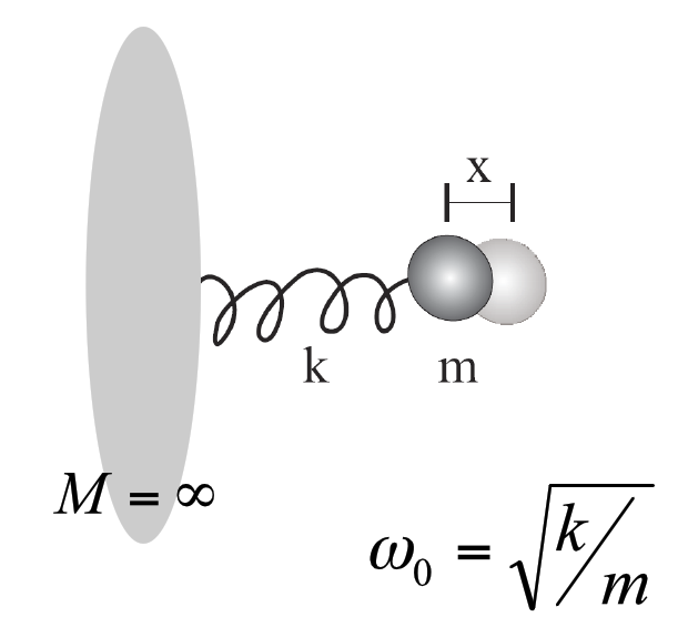
Once it’s disturbed a number of things begin to happen. First, it attempts to restore itself back to how it was before you disturbed it, and how quickly it does this is dictated by the spring constant 
Second, the way in which it restores itself depends to two properties: the mass 

When you have a system like this where you have two factors (disturbative and restorative) that are constantly pulling and pushing against each other, the position of the mass at any given time 


where 

So where did this equation come from? Long ago Newton did some work that allowed us to equate a force 

This is actually a second-order ordinary differential equation and this property becomes more apparent when acceleration is written as the second derivative of position with respect to time:

and one can re-arrange the two above equations so they look like a proper differential equation:

which has the solution 
It is interesting that mathematics says that the position of the mass under these conditions is dictated by a periodic, sinusoidal pattern. In other words, the mass will continue to oscillate up and down in a very periodic way and this position now can be described by 1) the initial displacement of the disturbance (the amplitude 

Energy
Now let’s talk about the mechanical energy 
The energy can always be expressed as the sum of two parts: the first being the kinetic energy and the second begin the potential energy. As we all know, a mass undergoing oscillatory motion will move between having only potential energy (at the peaks and troughs) and only kinetic energy (when it is moving the fastest, midway between the peaks and troughs) – all the while the sum of the two (the total energy of the system) remains perfectly constant.
These two components of total mechanical energy is given by

Further, it is well known that


where one would normally write 
Some Quantum Mechanics
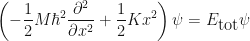
Let’s leave the SHO behind for a moment and recall the Schrödinger equation:

A couple of things here: The 

But this is ugly, and will probably scare a lot of people away.
Essentially, Schrödinger is telling us that the total energy 

and this is not at all like the total energy with potential and kinetic energy as written a couple of equations above – it’s got all these extra bits!
Where did they come from?
They come from re-writing the momentum 

On its own this doesn’t do much because it is differential operator – so it must operate on something. I haven’t told you yet what it operates (spoiler: wavefunctions), so regard this as a just an instruction for now.
Schrödinger’s equation just equates two different forms of total energy of a system. On the left is 
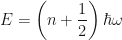
The Schrödinger equation has a solution as well, but you’re not going to like how we solve it but I promise that you will like the look of the final solution:
Isn’t that nice?
Looks more simple than you might expect.
This is saying that given some funny quantum stuff going on with the momentum part of the SHO (which we haven’t explained yet) the total energy of the (quantum) system is not continuous.
Well that is weird. Why?
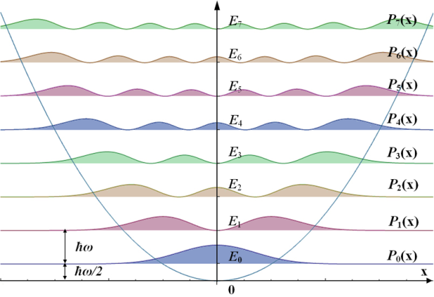
Because, as it is written, the energy of a SHO only has values for each integer 
The total energy is this integer number 
So we didn’t do anything wrong here. All we did was say that the momentum (related to the kinetic energy part of the SHO) was a bit funny (quantised). Once we did that, however, the total energy of the system suddenly stops being continuous and has all these integer values, like a ladder, and in between: simply does not exist!
So what does the 


For a mass of 


This value of this energy is called the zero point energy and, even though it clearly is not zero, it is still a very, very small amount of energy. This is not always the case though, there are systems where the zero point energy is actually zero, but not for a simple harmonic oscillator!
Our problem is that the SHO is a very simple system. It is so simple it shows up an awful lot in nature (nature likes simple things). For example, in quantum field theory, empty space is supposedly made up of an infinity of these tiny quantum simple harmonic oscillators. There are other overlapping fields too, like the fermionic and bosonic fields. Each of these are modelled as having a tiny SHO at each and every point in space. Given a forceful disturbance these fields can oscillate too (although damped) and when not oscillating they too have a zero point energy, and, you guessed it, since they are quantum they will have a non-zero energy (even though it’s called zero point energy!). At each point in space, the combination of all these fields contributes 
Er, isn’t this article about creation and annihilation?
How do we get the creation and annihilation operators from here? The trick is to consider Heisenberg’s uncertainty principle. His principle states that position

In other words, if you measure momentum 
The non-commutativity of the factorisation of the Hamiltonian of the quantum SHO is off by a factor of the zero point energy.
If we now go back to the quantum Hamiltonian

and put in the values of 


then factorise

(note: the 

When we expand we will inevitably get a 


and the bit on the right (
![\displaystyle H + \frac{1}{2}i\omega\left(xp - px\right) = H+\frac{1}{2}i\omega[x,p] = H+\frac{1}{2}i\omega(i\hbar) = H-\frac{1}{2}\hbar\omega = H - E_0 \neq H](https://s0.wp.com/latex.php?latex=%5Cdisplaystyle+H+%2B+%5Cfrac%7B1%7D%7B2%7Di%5Comega%5Cleft%28xp+-+px%5Cright%29+%3D+H%2B%5Cfrac%7B1%7D%7B2%7Di%5Comega%5Bx%2Cp%5D+%3D+H%2B%5Cfrac%7B1%7D%7B2%7Di%5Comega%28i%5Chbar%29+%3D+H-%5Cfrac%7B1%7D%7B2%7D%5Chbar%5Comega+%3D+H+-+E_0+%5Cneq+H&bg=%23ffffff&fg=%23111111&s=0&c=20201002)
OK, wow. This means a lot. The non-commutativity of the factorisation of the Hamiltonian of the quantum SHO is off by a factor of the zero point energy. The quantum-ness introduced in to the momentum 
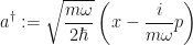
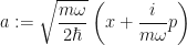
Now look at the factors in the parentheses (from a couple of equations back):


we call these the creation and annihilation operators 
![\displaystyle H = \frac{1}{2}m\omega^2\left[x^2 + \displaystyle\frac{1}{m^2\omega^2}p^2 \right]](https://s0.wp.com/latex.php?latex=%5Cdisplaystyle+H+%3D+%5Cfrac%7B1%7D%7B2%7Dm%5Comega%5E2%5Cleft%5Bx%5E2+%2B+%5Cdisplaystyle%5Cfrac%7B1%7D%7Bm%5E2%5Comega%5E2%7Dp%5E2+%5Cright%5D&bg=%23ffffff&fg=%23111111&s=0&c=20201002)
then factorising the part in the parentheses (not forgetting about the extra zero point energy bit):
![\displaystyle H = \frac{1}{2}m\omega^2\left[\left(x - \displaystyle \frac{i}{m\omega}p \right)\left( x + \displaystyle \frac{i}{m\omega}p \right) + \displaystyle \frac{\hbar}{m\omega^2}\right]](https://s0.wp.com/latex.php?latex=%5Cdisplaystyle+H+%3D+%5Cfrac%7B1%7D%7B2%7Dm%5Comega%5E2%5Cleft%5B%5Cleft%28x+-+%5Cdisplaystyle+%5Cfrac%7Bi%7D%7Bm%5Comega%7Dp+%5Cright%29%5Cleft%28+x+%2B+%5Cdisplaystyle+%5Cfrac%7Bi%7D%7Bm%5Comega%7Dp+%5Cright%29+%2B+%5Cdisplaystyle+%5Cfrac%7B%5Chbar%7D%7Bm%5Comega%5E2%7D%5Cright%5D+&bg=%23ffffff&fg=%23111111&s=0&c=20201002)
Substituting the symbols for the creation and annihilation operators, we simply equate together to two representations of the part inside the brackets to get:

A little re-arranging and we get:

We would prefer not to have the 
Where the bits out the front, 
![[x,p]](https://s0.wp.com/latex.php?latex=%5Bx%2Cp%5D&bg=%23ffffff&fg=%23111111&s=0&c=20201002)


And now, you must press the “I believe in Quantum Mechanics“-button (i.e. the Born postule) in which case fundamental relations between canonical conjugate quantities (like position and momentum) satisfy
![\displaystyle [x,p] = i\hbar](https://s0.wp.com/latex.php?latex=%5Cdisplaystyle+%5Bx%2Cp%5D+%3D+i%5Chbar+&bg=%23ffffff&fg=%23111111&s=0&c=20201002)
noting that ![(xp - px) = [x,p]](https://s0.wp.com/latex.php?latex=%28xp+-+px%29+%3D+%5Bx%2Cp%5D+&bg=%23ffffff&fg=%23111111&s=0&c=20201002)

Now we just need to substitute in the expression for the Hamiltonian 

A little rearranging and we get the main result of this article:
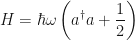
Whoa, whoa, hold on. This looks almost exactly the same as our solution to Schrödinger’s equation from the beginning of the article:

except that we have replaced 

This allows us to write:
![\displaystyle [a,a^{\dagger}] := aa^{\dagger} - a^{\dagger}a](https://s0.wp.com/latex.php?latex=%5Cdisplaystyle+%5Ba%2Ca%5E%7B%5Cdagger%7D%5D+%3A%3D+aa%5E%7B%5Cdagger%7D+-+a%5E%7B%5Cdagger%7Da+&bg=%23ffffff&fg=%23111111&s=0&c=20201002)
we have
![\displaystyle aa^{\dagger} = [a,a^{\dagger}] + a^{\dagger}a = 1 + a^{\dagger}a = 1 + N](https://s0.wp.com/latex.php?latex=%5Cdisplaystyle+aa%5E%7B%5Cdagger%7D+%3D+%5Ba%2Ca%5E%7B%5Cdagger%7D%5D+%2B+a%5E%7B%5Cdagger%7Da+%3D+1+%2B+a%5E%7B%5Cdagger%7Da+%3D+1+%2B+N&bg=%23ffffff&fg=%23111111&s=0&c=20201002)
Summary
We started with a very simple physical system: the simple harmonic oscillator (SHO) and used Newton’s second law to turn it in to a linear ordinary differential equation (ODE). Then we used kinetic and potential energy to write down the total energy of the system at any point.
Then we equated the total energy of the system to Schrödinger’s equation (essentially they should be the same, as they both express the energy of the system and they’re both differential equations) – and then made one important assumption: that momentum was quantised.
Once we did this we found that not only is the energy also quantised but also has a minimum called the zero-point energy.
Then we mixed in a little of Heisenberg’s Uncertainty principle and out popped two non-Hermitian operators
See Also
Chapter 9, Harmonic Oscillator, Nuclear Engineering at MIT.
References
[1] Lancaster, T & Blundell, S. J., Quantum Field Theory for the Gifted Amateur, Oxford University Press (2014)
