
In the previous article we got to grips with the fundamental behaviour of qubits by reviewing the historical account of regular bits. Qubits and Bits share a fundamental property: they are both two-state systems and the previous article focused on this, explaining that the bright minds of centuries past had figured out how to perform mathematical operations on pretty much any physical thing with two states.
A tremendous achievement.
But qubits are also two-state systems, so in exactly the same way for bits, they also store data and we can perform operations on them. The difference is that they also exhibit quantum properties.
But what is a quantum property? And how do we express them on paper?
Describing a quantum property requires the use of
Qubits Require Complex Numbers
Let’s think about why we need complex numbers to describe qubits. Essentially it boils down to the fact that rotation in the Euclidean plane using real numbers reduces to simple multiplication using complex numbers.
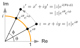
Multiplication is much, much easier to do than trigonometry, so the equations of quantum mechanics look and feel much simpler using complex numbers.
If you are not comfortable with complex numbers, fear not, I will try to reference them sparingly in what follows. If anything, just imagine complex numbers as pairs of real numbers that might describe a point on a map (e.g. latitude and longitude are both real numbers, the pair together describes a point on the Earth. That point is a complex number). In this example though, the longitude 


where that plus sign is vector addition and 
Complex numbers are what you get if you extend the real line above and below to infinity.
Complex numbers hold more information than real numbers. This is important, and is often referred to as an object’s degrees of freedom.
For example, a complex number has an extra property called phase denoted 


will always reduce to 
So, complex numbers have an additional degree of freedom, or as I like to say:
Complex numbers (over real numbers) have extra pockets you can put things in…
If you look at the very definition of a complex number 
where 


Now, look at the wikipedia definition of a pure qubit state:
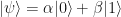
See the similarity!?
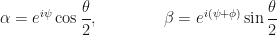
If qubits are necessarily linear combinations of some basis states 
Wait…shouldn’t there be four degrees of freedom? After all, each complex number 

Well, no. Quantum Theory is also a theory of probability. Which means we have a this axiom which forces us to constraint our system with the following relation:

which is called the normalisation constraint, and it removes a degree of freedom. In other words, you can write both 
…the so-called Hopf coordinates.
OK, but that’s still three. How do we get to two?
Well, we have that global phase component of the qubit: 

and this only has 2 variables, namely 

Since a qubit has 2 degrees of freedom, we can describe it using two coordinates in 2-dimensional space (a plane), hence the usefulness of using the Bloch Sphere to represent it:

But there is more to qubits than just looking like complex numbers…
Qubits Require Matrices
The reason why we need matrices is because of quantum logic gates and the fact that gates always have matrix representations. Furthermore, all binary Truth Tables (which we looked at in the previous article) can be expressed in the form of a square matrix known as a permutation matrix, putting even further emphasis on the need for using matrices.
So how do we go from
to a matrix?
Well, easy. We just write those basis states as vectors:

as
Storing Binary Data Using Logic Gates
Recall from the first article the logic gates of classical bits. For convenience, they are:
- NOT
- AND & NAND
- OR & NOR
- XOR & XNOR
Using these logic gates one can store binary data. How? By building a flip-flop.
Take a pair of NOR logic gates and cross-couple them, now you’ve got yourself a so-called set-reset latch which can store either a 0 or a 1 on a bit indefinitely – which is why, sometimes, flip-flops are called bi-stable circuits: which are circuits that have no charge or discharge time due to the absence of capacitors.
There are other flip-flops too, for example:
- Set-Reset NOR Latch
- Complement Set-Reset NAND Latch
- Set-Reset AND-OR Latch
- JK (Toggle) Latch
and there’s more.
If you arrange multiple flip-flops in parallel and you’ve got yourself a register. When a system is capable of performing flip-flops we say that the system has memory.
The point is: logic gates can store binary data – and the question is:
Can qubits store data?
Yes.
But we need qubit gates.
Gates for Qubits
Logic gates for qubits are unitary matrices.
Why?
Because for any time interval over which we are trying to realise a particular transformation (i.e. perform an experiment, or just crunch some numbers) we must use the Schrödinger equation (why? because we are working in quantum theory). This equation, necessarily involves Hamiltonians which, are required to be Hermitian (or self-adjoint) to yield real-world results. This condition of Hermiticity implies that the transformation is unitary.
Because there are more degrees of freedom in a qubit (namely 2, instead of 1 for a classical bit) a quantum logic gate is not only a unitary matrix, it is also a square matrix of size 
When you act on a 


But this can always be represented in terms of the standard basis:

The Linear Shift of the QFT
We have used the Quantum Fourier Transform (QFT) before in this article here. Let’s now see the raw power of the qubit by performing a QFT on it.
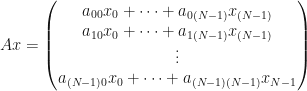
In 
Then linear algebra states that the matrix multiplication of a matrix 

The QFT is a quantum gate, thus, it is a unitary matrix.
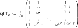
We can apply the unitary QFT on it via matrix multiplication on the basis representation:

Let’s do the first multiplication:

Summary
A computer contains a bunch of physical components, such as gears and cams in mechanical computers, relays and switches in classical computers, and transistors in modern computers. In the mechanical computer the physical state is the rotational orientation of the gears, in the classical computer it is the binary on or off state of the relay, and in the modern computer it is the current and voltage in the transistor.
Physical interactions between these components, causing them to change their state, achieves computation. In the modern computer, data (voltages and current) from memory circuits is transferred to the central processing unit (CPU) where they interact with logic gates (such as AND and OR) implemented in series and parallel, producing new voltages and new currents (a.k.a. the output) which can then be stored back in memory circuits and, ultimately, read (or measured) by the user.
References
[1] https://courses.edx.org/c4x/BerkeleyX/CS191x/asset/chap5.pdf
[2] Nielsen, N. & Chuang, I. L. – Quantum Computation and Quantum Information, Cambridge University Press, (2010).

I just discovered your blog, it seems great, I am checking articles…
But, in this one, just before the summary, in the “Let’s do the first multiplication”, I get a “Formula does not parse” in the latex formula… could you fix it, please?