
In this last article we attempted to motivate the use of the Quantum Fourier Transform (QFT) in a quantum circuit by looking at what happens when we assume:
- a unitary operator, and
- exactly
qubits
Then we could then factor the unitary operator as

We then extended the unitary operator in to a controlled unitary and noticed that it has the exact same form as the controlled phase gate 


With the Hadamard gate 

which is nothing but:
which is the mathematical represention of the discrete Fourier transform!
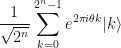
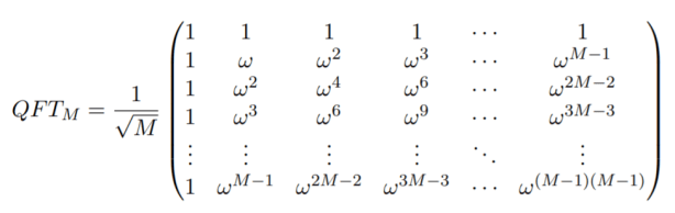
Then, in this article, we derived the actual matrix representation of the QFT. Here is what it looks like for a resgister of 4 qubits:
Notice that the first row and the first column are filled with 1’s? This is always the case for the QFT of any dimension; a property which is very often utilised in linear algebra calculations.
So how do we use this?
Well, let’s say that we have two quantum registers that differ only in their relative positions. We indicate this by permuting the indices of the individual qubits:

Now look what happens when we apply the QFT to them:
and
All the indices line up again!!!
The difference between the two outputs crucially only differs by a relative phase shift (see the ordering of the 

The phase of the state does not effect the probability of measuring that state.
As another illustrative example, imagine that we have the following two physically identical states:

What do you think will happen to these qubits?
It turns out that, even though they are physically identical, the application of the QFT on each of these does result in different outputs!


What on Earth is going on!?
Somehow we can have two physically identical states but physically different Fourier transformed states. While also having two physically different states but physically identical Fourier transformed states.
Confused?
It appears that the QFT is sensitive to some hidden characteristics of a register of qubits, while being completely indifferent to others.
We will exploit this behaviour of the QFT in what follows. But we will also need to know what are these characteristics.
The Algorithm
So how can an algorithm find prime factors?
Well, there are many classical algorithms which do the job just fine (although slowly) and they’ve been around for a long time. For example, the quadratic sieve or the general number field sieve (the fastest known classical algorithm), which uses a few simplifying assumptions (like 

These are all classical algorithms – and not the subject of this article. Suffice it to say: those algorithms are all very well known and work rather well. I would say that the only weakness in the classical algorithms is in the subroutine that attempts the find the period of the function 
The faster the algorithm can preclude more and more
Thus, if the algorithm finds out that 

This further testing is when we need to figure out the period of

If it turns out that the period is odd then the
It is in the figuring out the order of this periodic function where the quantum Fourier transform comes in. Everything else, stays classical.
Using the QFT to Find the Order of a Periodic Function
So, how does the QFT help us find the period of a periodic function?
First, note that there are many ways to factor an integer besides reducing factoring to period-finding.
In the last section above we showed that we can easily find a factor of
Classical computers suffer badly when trying to figure out the order of a function because they have to check each candidate one after the other until a success is found.
Even and Odd Functions
All right, let’s step back for a second and recall what even and odd functions are.
Two things can happen when you try to compute a shift in the argument of a function: 


Further, if the function is periodic and 


A function is odd if it changes sign when the argument is negative: 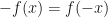
Even and Odd do not cover all examples of periodic functions. There are a huge number of functions which are neither even nor odd. Yet, it is very easy to test if a function is even or odd: just substitute 

Primitive Roots of Unity
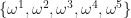
The last tool we need in our toolbox is the concept of a primitive root of unity. Recall that with the complex numbers there always exists

For example, if 


As such, it is much easier to write the solutions for 


In this language, when 
If you want to know specifically what, say, 

Graphically, these solutions all lie on the unit circle (hence the name):
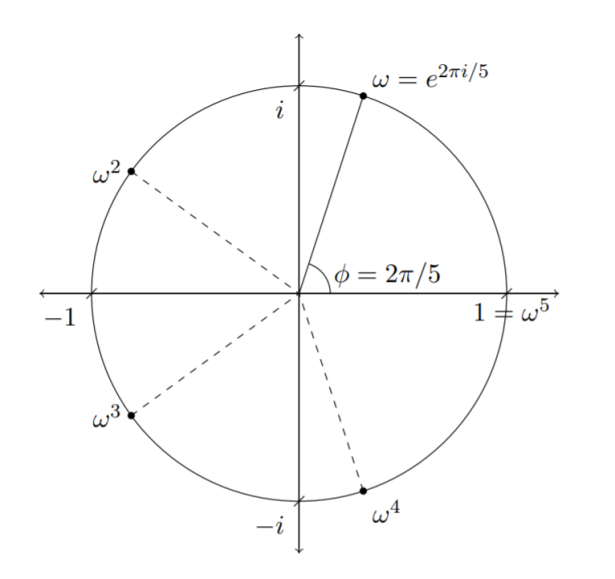
and they are all equally spaced apart.
The Discrete Fourier Transform
We’ve already seen in past articles that the QFT can be written in matrix form for any dimension 
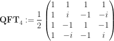
The 2-dimensional QFT (i.e. with 

But since 

is just the 2-dimensional Hadamard gate!
Indeed, the QFT is a generalisation of the Hadamard gate.
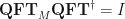
The QFT is also unitary because its columns are all pairwise orthonormal. This also means that whenever you perform the QFT and then its adjoint, you get the identity operator:
Period Finding
What is period finding?
Well, suppose you have a periodic function (e.g. 


But what if I said that 
No it doesn’t…
Oh, but it does… in modulo
In fact, all of those
Periodic functions and arguments equalling one another in some modulo are equivalent statements:
A periodic function has the property that
if and only if

In our case, the remainder 

We can already classically find the period
Very slow.
In fact, as the dimensionality 
With quantum computers though, we can place 
If we take our register of 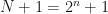
![\displaystyle |0\rangle^{\otimes N}|0\rangle \xrightarrow[]{\mathbf{QFT}_N} \frac{1}{\sqrt{N}} \sum_{x=0}^{N-1} |x\rangle|0\rangle](https://s0.wp.com/latex.php?latex=%5Cdisplaystyle+%7C0%5Crangle%5E%7B%5Cotimes+N%7D%7C0%5Crangle+%5Cxrightarrow%5B%5D%7B%5Cmathbf%7BQFT%7D_N%7D+%5Cfrac%7B1%7D%7B%5Csqrt%7BN%7D%7D+%5Csum_%7Bx%3D0%7D%5E%7BN-1%7D+%7Cx%5Crangle%7C0%5Crangle&bg=%23ffffff&fg=%23111111&s=0&c=20201002)
Now, we transform our ancilliary zero-state according to some unitary operator 
![\displaystyle |0\rangle^{\otimes N}|0\rangle \xrightarrow[]{U_f} \frac{1}{\sqrt{N}} \sum_{x=0}^{N-1} |x\rangle|f(x) \rangle](https://s0.wp.com/latex.php?latex=%5Cdisplaystyle+%7C0%5Crangle%5E%7B%5Cotimes+N%7D%7C0%5Crangle+%5Cxrightarrow%5B%5D%7BU_f%7D+%5Cfrac%7B1%7D%7B%5Csqrt%7BN%7D%7D+%5Csum_%7Bx%3D0%7D%5E%7BN-1%7D+%7Cx%5Crangle%7Cf%28x%29+%5Crangle&bg=%23ffffff&fg=%23111111&s=0&c=20201002)
If we then decide to measure the ancilliary state 


But that’s not so bad, because we know that 
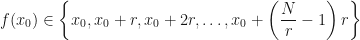
Which means the pre-image must contain some set of 
So, our measurement makes this change:
![\displaystyle \frac{1}{\sqrt{N}}\sum_{x=0}^{N-1}|x\rangle|f(x)\rangle \xrightarrow[]{\textup{measure}} \frac{1}{\sqrt{N}} \sum_{x=0}^{N-1} \left|\left( x_0 + \left(\frac{N}{r} - 1\right)r\right)\right\rangle|f(x_0) \rangle](https://s0.wp.com/latex.php?latex=%5Cdisplaystyle+%5Cfrac%7B1%7D%7B%5Csqrt%7BN%7D%7D%5Csum_%7Bx%3D0%7D%5E%7BN-1%7D%7Cx%5Crangle%7Cf%28x%29%5Crangle+%5Cxrightarrow%5B%5D%7B%5Ctextup%7Bmeasure%7D%7D+%5Cfrac%7B1%7D%7B%5Csqrt%7BN%7D%7D+%5Csum_%7Bx%3D0%7D%5E%7BN-1%7D+%5Cleft%7C%5Cleft%28+x_0+%2B+%5Cleft%28%5Cfrac%7BN%7D%7Br%7D+-+1%5Cright%29r%5Cright%29%5Cright%5Crangle%7Cf%28x_0%29+%5Crangle&bg=%23ffffff&fg=%23111111&s=0&c=20201002)

The astute reader will notice that the summation has narrowed, and we will be just ignoring the last
Now our register is in a periodic superposition where its period is equal to the period of the function 
But we can’t measure it just yet! This is because when we run this algorithm up to this point we might measure a different value of 
The QFT again comes to our rescue.
Recall that if a function 


Further, recall that when this happens, any constant linear shift inherent in the function is transformed in to the phase of
The Quantum Fourier Transform not only transforms periods of the form
to
Therefore, if we take the QFT of the first register, we will be left with only the states that are multiples of 
Applying the QFT again to the first
![\displaystyle \sqrt{\frac{r}{N}}\sum_{j=0}^{\frac{N}{r}-1} |x_0 + jr \rangle \xrightarrow[]{\mathbf{QFT}} \frac{1}{\sqrt{r}} \sum_{j=0}^{r-1} \omega^j \left| i \frac{N}{r} \right\rangle](https://s0.wp.com/latex.php?latex=%5Cdisplaystyle+%5Csqrt%7B%5Cfrac%7Br%7D%7BN%7D%7D%5Csum_%7Bj%3D0%7D%5E%7B%5Cfrac%7BN%7D%7Br%7D-1%7D+%7Cx_0+%2B+jr+%5Crangle+%5Cxrightarrow%5B%5D%7B%5Cmathbf%7BQFT%7D%7D+%5Cfrac%7B1%7D%7B%5Csqrt%7Br%7D%7D+%5Csum_%7Bj%3D0%7D%5E%7Br-1%7D+%5Comega%5Ej+%5Cleft%7C+i+%5Cfrac%7BN%7D%7Br%7D+%5Cright%5Crangle+&bg=%23ffffff&fg=%23111111&s=0&c=20201002)
where 

We can now measure and retrieve 
We repeat this algorithm and measure to retrieve several multiples of
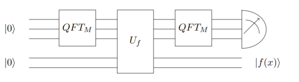
This algorithm can be summed up by the following circuit:
Example
OK, I understand all of that was pretty high-brow, and probably didn’t make a whole lot of sense. So let us go through a concrete example.
Suppose we define a periodic function 
Let’s use a 3-qubit system, so that 

First, let’s apply the QFT. The QFT of 3 qubits is the 
![\displaystyle |0\rangle^{\otimes 3}|0\rangle \xrightarrow[]{\mathbf{QFT}_8} \frac{1}{\sqrt{8}}\sum_{x=0}^7 |x\rangle|0\rangle](https://s0.wp.com/latex.php?latex=%5Cdisplaystyle+%7C0%5Crangle%5E%7B%5Cotimes+3%7D%7C0%5Crangle+%5Cxrightarrow%5B%5D%7B%5Cmathbf%7BQFT%7D_8%7D+%5Cfrac%7B1%7D%7B%5Csqrt%7B8%7D%7D%5Csum_%7Bx%3D0%7D%5E7+%7Cx%5Crangle%7C0%5Crangle&bg=%23ffffff&fg=%23111111&s=0&c=20201002)
Now we apply our unitary function:
![\displaystyle \frac{1}{\sqrt{8}}\sum_{x=0}^7 |x\rangle|0\rangle \xrightarrow[]{U_f} \frac{1}{\sqrt{8}}\sum_{x=0}^7 |x\rangle|f(x) \rangle](https://s0.wp.com/latex.php?latex=%5Cdisplaystyle+%5Cfrac%7B1%7D%7B%5Csqrt%7B8%7D%7D%5Csum_%7Bx%3D0%7D%5E7+%7Cx%5Crangle%7C0%5Crangle+%5Cxrightarrow%5B%5D%7BU_f%7D+%5Cfrac%7B1%7D%7B%5Csqrt%7B8%7D%7D%5Csum_%7Bx%3D0%7D%5E7+%7Cx%5Crangle%7Cf%28x%29+%5Crangle&bg=%23ffffff&fg=%23111111&s=0&c=20201002)
Before continuing, let is peek inside and see what the state looks like:
![\displaystyle \frac{1}{\sqrt{8}}\sum_{x=0}^7 |x\rangle|f(x) \rangle \xrightarrow[]{\textup{measure }|f(x)\rangle } \frac{1}{2}(|1\rangle + |3\rangle + |5\rangle + |7\rangle)\otimes|1\rangle](https://s0.wp.com/latex.php?latex=%5Cdisplaystyle+%5Cfrac%7B1%7D%7B%5Csqrt%7B8%7D%7D%5Csum_%7Bx%3D0%7D%5E7+%7Cx%5Crangle%7Cf%28x%29+%5Crangle+%5Cxrightarrow%5B%5D%7B%5Ctextup%7Bmeasure+%7D%7Cf%28x%29%5Crangle+%7D+%5Cfrac%7B1%7D%7B2%7D%28%7C1%5Crangle+%2B+%7C3%5Crangle+%2B+%7C5%5Crangle+%2B+%7C7%5Crangle%29%5Cotimes%7C1%5Crangle+&bg=%23ffffff&fg=%23111111&s=0&c=20201002)
OK, so that is interesting. All those qubit states are odd. Measuring this state of this register will yield a 1, 3, 5 or 7 with equal probability of 25%. So a sequence of measurements might look like this: 31755713357137735731355753135753137771573573171735… which is just a random sequence of integers. How do we get the number 2 from this?
Well, we can’t just yet. So we once again apply the QFT:
![\displaystyle \frac{1}{2}(|1\rangle + |3\rangle + |5\rangle + |7\rangle) \xrightarrow[]{\mathbf{QFT}_8} \frac{1}{\sqrt{2}}(|0\rangle + |4\rangle)](https://s0.wp.com/latex.php?latex=%5Cdisplaystyle+%5Cfrac%7B1%7D%7B2%7D%28%7C1%5Crangle+%2B+%7C3%5Crangle+%2B+%7C5%5Crangle+%2B+%7C7%5Crangle%29+%5Cxrightarrow%5B%5D%7B%5Cmathbf%7BQFT%7D_8%7D+%5Cfrac%7B1%7D%7B%5Csqrt%7B2%7D%7D%28%7C0%5Crangle+%2B+%7C4%5Crangle%29+&bg=%23ffffff&fg=%23111111&s=0&c=20201002)
Note: if instead of measuring 

![\displaystyle \frac{1}{2}(|0\rangle + |2\rangle + |4\rangle + |6\rangle) \xrightarrow[]{\mathbf{QFT}_8} \frac{1}{\sqrt{2}}(|0\rangle + |4\rangle)](https://s0.wp.com/latex.php?latex=%5Cdisplaystyle+%5Cfrac%7B1%7D%7B2%7D%28%7C0%5Crangle+%2B+%7C2%5Crangle+%2B+%7C4%5Crangle+%2B+%7C6%5Crangle%29+%5Cxrightarrow%5B%5D%7B%5Cmathbf%7BQFT%7D_8%7D+%5Cfrac%7B1%7D%7B%5Csqrt%7B2%7D%7D%28%7C0%5Crangle+%2B+%7C4%5Crangle%29+&bg=%23ffffff&fg=%23111111&s=0&c=20201002)
See how the answer is still 
So now we are getting somewhere. Now, no matter what the function 

Now we definitely can extract the number 2 from this.
Taking the largest value (which is 4) we can solve the equation 

In this case, 


and so the coefficient was 
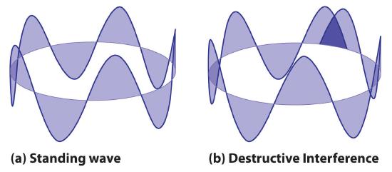
It should be clear by now that we get this coeffcient due to the constructive interference in rotations around the unit circle. When 
Additions in the phase of the qubit state create constructive and destructive interference, cancelling and enhancing the probabilities of observing the correct quantum state upon measurement after performing a quantum Fourier transform.
Summary
We saw how a QFT is sensitive to the phase-structure of a register of qubits. Just because a register of qubits is physically identical to another is not enough to ensure the QFT of those registers will be identical. Small differences is the unobservable, unphysical global phases can wildly affect the outcome of the QFT. But by the same token, some states will be identical under a QFT, and we took advantage of this when we mapped the different result sets of
We then found a way to programmatically turn a function in to a binary test, by determining whether or not it is an even or an odd function – a binary outcome.
Then we found a connection between the primitive roots of unity and the matrix elements that make up the unitary QFT. We saw that the simplest QFT is, in fact, just the Hadamard transform. Higher-dimensional QFTs are just unitary matrices of rotations in the complex plane, just as products of primitive roots of unity are.

We then came to the problem of period finding. By first placing a register of qubits in to a superposition (via a QFT as a generalised Hadamard), we then apply the periodic function whose period we seek as a unitary transformation on the superpositioned register of qubits. By the definition of periodic, if we make a measurement here, we know the qubit states must collapse in to one of the periodic values, but not necessarily the largest one that we seek. We can increase the probability of finding the right one by applying the QFT again (and in this case, not necessarily as a Hadamard but as a way to provide destructive and constructive interference in the global phases of the superpositioned qubits, so that the final measurement will have a higher likelihood of being the period that we seek.
As a circuit we just described doing this:
References
[1] Cleve, Ekert, Macchiavello, Mosca – Quantum algorithms revisited, Proceedings of the Royal Society 454 (1998).
[2] Nielsen, N. & Chuang, I. L. – Quantum Computation and Quantum Information, Cambridge University Press, (2010).
[3] Kendon, V. M. & Munro, W. J. – Entanglement and its Role in Shor’s algorithm, arXiv:quant-ph/0412140 (2006).
[4] Jozsa, R. – Quantum factoring, discrete logarithms and the hidden subgroup problem, arXiv:quant-ph/0012084 (2001).
[5] Cleve, R., Ekert, A., Macchiavello, C., & Mosca, M., – Quantum Algorithms Revisited, (1997)
