
How do you get from this:
to this:
?
Welcome to the 5th article in my series on Quantum Computing.
In the last article we spent the majority of our time setting up Qiskit in PyCharm. We encountered a couple of hurdles along the way (like getting Qiskit to generate charts), but in the end we managed to get it all working – but didn’t really do any quantum programming. That’s about to change.
The problem is, we don’t have any tools to convert mathematical operations in to equivalent quantum circuits. I know we had a brief look at how this was done for addition on classical circuits, but did you know that even addition is forbidden in quantum circuits? More on that later.
Instead, we are going to look at a different mathematical operation known as a fourier transform and see if we can get it constructed in to a quantum circuit.
This will require quite a bit of math. But if you can get through it, I guarantee you will feel a lot better about this step in the process of quantum computing. In fact, I think this step in particular, separates those who think they know how quantum circuits work and those that do.
This article will involve a range of more advanced topics but, like before, I will introduce each one very slowly. If you are not comfortable with the tensor product representation of a many-qubit state basis vector, you will have to brush up on that. We will also need to be familiar with the Hadamard gate and the Rotation gates. We will be working in the Fourier-transformed amplitude space, so a lot of the calculations will be rotations in the complex plane – get ready for a lot of complex exponentials. There will also be a large component that needs to be converted in to binary (so that we can see exactly how each input qubit maps to an output qubit). For this we will be delving in to the realm of fractional binary notation.
Lastly, we will finish this article off by theoretically building a circuit – yes, we will be going all the way from the Fourier Transform to an actual quantum circuit. In the next article we will implement the circuit in Qiskit’s Aqua in Python.
The Quantum Fourier Transform Circuit
What is the Quantum Fourier Transform (QFT)?
First, it is a linear transformation – which means that it preserves addition and multiplication by scalars; and that it can also be used in quantum circuits (all quantum operations must be linear).
But this is nothing special, many interesting maps are linear. So what else?
Well, it’s unitary. OK, that’s particularly useful for quantum programming, it means it has a Hermitian adjoint. It also has a matrix representation. Also cool. But what does it actually do?
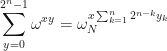
It maps vectors to funny-looking vectors:
That looks ugly and there are a lot of letters in there to explain. First, it involves a summation over 


which is a rotation, and so the map looks like this:
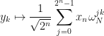
and so it is clear that the QFT is rotating something around something.
What else can we do?
Well, we can use qubit notation for a basis state 

Note how 

Therefore, if we have a 3-qubit system, the QFT would map a basis vector like this:

and therefore, even though we only have 3 qubits, we will need an 
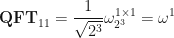
Let’s see what the matrix representation of this 3-qubit system looks like:
For the first row, the first entry would be:

The second entry would be:

In fact, every entry along the first row is 1 due to the presence of the zero in the exponent.
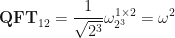
Moving on to the second row. The first element would be:

The second element on the second row:
The third element:
Continuing in this way, we arrive at the full matrix representation of the QFT:

This bulky matrix can be simplified using a bit of algebra. Note that since 


Since we are working with eighths (i.e. 


Furthermore, we can reduce rotations to modulo 8, i.e. if we see a 

The resulting matrix for QFT is:

This is what you would call a concrete example of a QFT matrix. What we need is an generalised version of this matrix that holds for any number of qubits. Only then will we be able to see how to manipulate it for any scenario.
The General Matrix Representation
We know that the outer product of two state vectors produces a matrix. We also know that with the QFT we have the input state vector 


This matrix will compute the entries of the associated 
But is it Unitary?
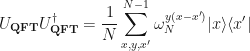
It is easy to show that the QFT is unitary, and, in fact, it is customary to denote it by 
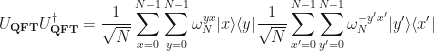
Writing it this way lets us put 


Now, the delta function 

But now the rotation 

And, again, the delta function is going to turn any 
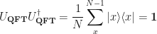
Therefore, the QFT matrix is unitary.
The QFT as a Quantum Circuit
Deriving a quantum circuit for the 3-qubit case is a little difficult to start with. Let’s go back to the 2-qubit case (remember, that means a 

Can we do anything with this expression? Well, a quantum circuit is qubit-dependent i.e. we will need to know exactly what to do with each qubit if we want to implement a QFT. Therefore, those state vectors in the above representation for a QFT will need to be expanded:
Here we have split out the target state vector as a product of states (standard stuff):

and therefore, the product in the exponent becomes a sum:

But because the original sum goes to 

Now for each 


…and there would be

Rearranging the sum and product
Since 


To get:

Expanding the Product Using Fractional Binary Notation
We would like to now expand the
The definition of the binary fraction is this:
![\displaystyle [0.x_1\cdots x_m] := \sum_{j=1}^m x_j 2^{-j}](https://s0.wp.com/latex.php?latex=%5Cdisplaystyle+%5B0.x_1%5Ccdots+x_m%5D+%3A%3D+%5Csum_%7Bj%3D1%7D%5Em+x_j+2%5E%7B-j%7D+&bg=%23ffffff&fg=%23111111&s=0&c=20201002)
To see how this is used it is extremely useful to compute some examples. Consider first ![[0.x_1]](https://s0.wp.com/latex.php?latex=%5B0.x_1%5D&bg=%23ffffff&fg=%23111111&s=0&c=20201002)


![\displaystyle [0.x_1] := \sum_{j=1}^1 x_j 2^{-j} = x_1 2^{-1} = \frac{x_1}{2}](https://s0.wp.com/latex.php?latex=%5Cdisplaystyle+%5B0.x_1%5D+%3A%3D+%5Csum_%7Bj%3D1%7D%5E1+x_j+2%5E%7B-j%7D+%3D+x_1+2%5E%7B-1%7D+%3D+%5Cfrac%7Bx_1%7D%7B2%7D+&bg=%23ffffff&fg=%23111111&s=0&c=20201002)
Pretty simple. What about ![[0.x_1 x_2]](https://s0.wp.com/latex.php?latex=%5B0.x_1+x_2%5D&bg=%23ffffff&fg=%23111111&s=0&c=20201002)

![\displaystyle [0.x_1x_2] := \sum_{j=1}^2 x_j 2^{-j} = x_1 2^{-1} + x_2 2^{-2} = \frac{x_1}{2}+\frac{x_2}{4}](https://s0.wp.com/latex.php?latex=%5Cdisplaystyle+%5B0.x_1x_2%5D+%3A%3D+%5Csum_%7Bj%3D1%7D%5E2+x_j+2%5E%7B-j%7D+%3D+x_1+2%5E%7B-1%7D+%2B+x_2+2%5E%7B-2%7D+%3D+%5Cfrac%7Bx_1%7D%7B2%7D%2B%5Cfrac%7Bx_2%7D%7B4%7D+&bg=%23ffffff&fg=%23111111&s=0&c=20201002)
Again, pretty simple.
Things get a little more tricky with ![[0.x_n]](https://s0.wp.com/latex.php?latex=%5B0.x_n%5D&bg=%23ffffff&fg=%23111111&s=0&c=20201002)
![\displaystyle [0.x_n] := \sum_{j=n}^1 x_j 2^{-j} = x_n 2^{-n} = \frac{x_n}{2^n}](https://s0.wp.com/latex.php?latex=%5Cdisplaystyle+%5B0.x_n%5D+%3A%3D+%5Csum_%7Bj%3Dn%7D%5E1+x_j+2%5E%7B-j%7D+%3D+x_n+2%5E%7B-n%7D+%3D+%5Cfrac%7Bx_n%7D%7B2%5En%7D+&bg=%23ffffff&fg=%23111111&s=0&c=20201002)
What about ![[0.x_{n-1} x_n]](https://s0.wp.com/latex.php?latex=%5B0.x_%7Bn-1%7D+x_n%5D&bg=%23ffffff&fg=%23111111&s=0&c=20201002)

![\displaystyle [0.x_{n-1}x_n] := \sum_{j=n-1}^2 x_j 2^{-j} = x_{n-1} 2^{-(n-1)} + x_n 2^{-n} = \frac{x_{n-1}}{2^{n+1}}+\frac{x_n}{2^n}](https://s0.wp.com/latex.php?latex=%5Cdisplaystyle+%5B0.x_%7Bn-1%7Dx_n%5D+%3A%3D+%5Csum_%7Bj%3Dn-1%7D%5E2+x_j+2%5E%7B-j%7D+%3D+x_%7Bn-1%7D+2%5E%7B-%28n-1%29%7D+%2B+x_n+2%5E%7B-n%7D+%3D+%5Cfrac%7Bx_%7Bn-1%7D%7D%7B2%5E%7Bn%2B1%7D%7D%2B%5Cfrac%7Bx_n%7D%7B2%5En%7D+&bg=%23ffffff&fg=%23111111&s=0&c=20201002)
With this little tool in mind, let’s now return to this guy:
Let’s expand the product in our minds and just consider what the last term would look like expanded out, recalling that 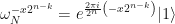

…and we can see that the last part of the exponential (the 
![\displaystyle |0\rangle + \exp\left(\frac{2\pi i}{2^n} x_n 2^{n-n}\right)|1\rangle = |0\rangle + \exp\left(2\pi i [0.x_n]\right)](https://s0.wp.com/latex.php?latex=%5Cdisplaystyle+%7C0%5Crangle+%2B+%5Cexp%5Cleft%28%5Cfrac%7B2%5Cpi+i%7D%7B2%5En%7D+x_n+2%5E%7Bn-n%7D%5Cright%29%7C1%5Crangle+%3D+%7C0%5Crangle+%2B+%5Cexp%5Cleft%282%5Cpi+i+%5B0.x_n%5D%5Cright%29+&bg=%23ffffff&fg=%23111111&s=0&c=20201002)
But there are

Taking a common factor of 

Which, the last part in parentheses has binary form: ![\frac{x_{n-1}}{2^{n+1}}+\frac{x_{n}}{2^{n}} = [0.x_{n-1}x_n]](https://s0.wp.com/latex.php?latex=%5Cfrac%7Bx_%7Bn-1%7D%7D%7B2%5E%7Bn%2B1%7D%7D%2B%5Cfrac%7Bx_%7Bn%7D%7D%7B2%5E%7Bn%7D%7D+%3D+%5B0.x_%7Bn-1%7Dx_n%5D&bg=%23ffffff&fg=%23111111&s=0&c=20201002)
![\displaystyle = |0\rangle + \exp\left(2\pi i [0.x_{n-1}x_n]\right)|1\rangle](https://s0.wp.com/latex.php?latex=%5Cdisplaystyle%C2%A0+%3D+%7C0%5Crangle+%2B+%5Cexp%5Cleft%282%5Cpi+i+%5B0.x_%7Bn-1%7Dx_n%5D%5Cright%29%7C1%5Crangle+&bg=%23ffffff&fg=%23111111&s=0&c=20201002)
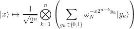
Continuing in the fashion all the way back to the first term we find a pattern of implementing longer and longer binary representations of the exponent. Eventually we get the full binary representation of the Quantum Fourier Transform:
![U_{\mathbf{QFT}}(|x_1 x_2 \cdots x_n\rangle) = \frac{1}{\sqrt{N}} \left( \left( |0\rangle + \exp\left(2\pi i [0.x_1x_2\dots x_n]\right)|1\rangle\right) \otimes \right.](https://s0.wp.com/latex.php?latex=U_%7B%5Cmathbf%7BQFT%7D%7D%28%7Cx_1+x_2+%5Ccdots+x_n%5Crangle%29+%3D+%5Cfrac%7B1%7D%7B%5Csqrt%7BN%7D%7D+%5Cleft%28+%5Cleft%28+%7C0%5Crangle+%2B+%5Cexp%5Cleft%282%5Cpi+i+%5B0.x_1x_2%5Cdots+x_n%5D%5Cright%29%7C1%5Crangle%5Cright%29+%5Cotimes+%5Cright.+&bg=%23ffffff&fg=%23111111&s=0&c=20201002)
![\displaystyle \quad\quad\quad \left.\cdots \otimes \left( |0\rangle + \exp\left(2\pi i [0.x_{n-1}x_n]\right)|1\rangle\right) \otimes \left( |0\rangle + \exp\left(2\pi i [0.x_n]\right)|1\rangle\right)\right)](https://s0.wp.com/latex.php?latex=%5Cdisplaystyle+%5Cquad%5Cquad%5Cquad+%5Cleft.%5Ccdots+%5Cotimes+%5Cleft%28+%7C0%5Crangle+%2B+%5Cexp%5Cleft%282%5Cpi+i+%5B0.x_%7Bn-1%7Dx_n%5D%5Cright%29%7C1%5Crangle%5Cright%29+%5Cotimes+%5Cleft%28+%7C0%5Crangle+%2B+%5Cexp%5Cleft%282%5Cpi+i+%5B0.x_n%5D%5Cright%29%7C1%5Crangle%5Cright%29%5Cright%29+&bg=%23ffffff&fg=%23111111&s=0&c=20201002)
This is a very useful form of the QFT for, specifically (and don’t forget!) the case where the number of qubits is some power of two, i.e. for 
Why?
The Most Important Result of this Article
Because take a look at that first qubit:
![\displaystyle \frac{1}{\sqrt{N}} \left( |0\rangle + \exp\left(2\pi i [0.x_1x_2\dots x_n]\right)|1\rangle\right)](https://s0.wp.com/latex.php?latex=%5Cdisplaystyle+%5Cfrac%7B1%7D%7B%5Csqrt%7BN%7D%7D+%5Cleft%28+%7C0%5Crangle+%2B+%5Cexp%5Cleft%282%5Cpi+i+%5B0.x_1x_2%5Cdots+x_n%5D%5Cright%29%7C1%5Crangle%5Cright%29&bg=%23ffffff&fg=%23111111&s=0&c=20201002)
It’s the ONLY one that depends on ALL values of all the other input qubits 
![\exp\left( -2\pi i[0.a] \right)](https://s0.wp.com/latex.php?latex=%5Cexp%5Cleft%28+-2%5Cpi+i%5B0.a%5D+%5Cright%29&bg=%23ffffff&fg=%23111111&s=0&c=20201002)


Combining What We Know to Build a Circuit
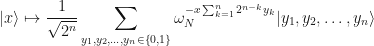
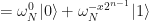
We already know that the Hadamard gate produces the following in a circuit of 
![\displaystyle |x\rangle \mapsto \frac{1}{\sqrt{2}} \left( |0\rangle + \exp\left( -2\pi i [0.x_1]\right)|1\rangle\right)\otimes|x_2, x_3, \dots, x_n\rangle](https://s0.wp.com/latex.php?latex=%5Cdisplaystyle+%7Cx%5Crangle+%5Cmapsto+%5Cfrac%7B1%7D%7B%5Csqrt%7B2%7D%7D+%5Cleft%28+%7C0%5Crangle+%2B+%5Cexp%5Cleft%28+-2%5Cpi+i+%5B0.x_1%5D%5Cright%29%7C1%5Crangle%5Cright%29%5Cotimes%7Cx_2%2C+x_3%2C+%5Cdots%2C+x_n%5Crangle+&bg=%23ffffff&fg=%23111111&s=0&c=20201002)
Note how the 
We also know that the Rotation Gate (a.k.a Phase Shift Gate) is

If we now apply controlled rotation gates 
![\displaystyle |x\rangle \mapsto \frac{1}{\sqrt{2}} \left( |0\rangle + \exp\left( -2\pi i [0.x_1x_2\dots x_n]\right)|1\rangle\right)\otimes|x_2, x_3, \dots, x_n\rangle](https://s0.wp.com/latex.php?latex=%5Cdisplaystyle+%7Cx%5Crangle+%5Cmapsto+%5Cfrac%7B1%7D%7B%5Csqrt%7B2%7D%7D+%5Cleft%28+%7C0%5Crangle+%2B+%5Cexp%5Cleft%28+-2%5Cpi+i+%5B0.x_1x_2%5Cdots+x_n%5D%5Cright%29%7C1%5Crangle%5Cright%29%5Cotimes%7Cx_2%2C+x_3%2C+%5Cdots%2C+x_n%5Crangle+&bg=%23ffffff&fg=%23111111&s=0&c=20201002)
and we have perfectly reproduced the first term of the above, expanded QFT state.
Then we move to the next qubit, perform another Hadmard, then the appropriate (one fewer) rotation gates, to get the second qubit.
Do this all the way to the end and you have effectively (in binary) produced the logical output of a Fourier transform on
This is what it looks like on a circuit diagram:
Summary
In this article we made the giant leap to being able to actually come up with a quantum circuit, at least in theory, starting from a mathematical equation. We had to expand and break up the Fourier transform equation in to bite size pieces, crucially by using its linearity and unitary properties. From here we needed to find a suitable ordering of the embedded product and sums and then re-expand it in binary to get at the individual qubits.
Once we got to that point all we had to do was notice that we were really just looking at a sequence of Hadamard and Rotation transformations! This is particularly easy to do when you have expressed your equation in binary notation.
In the next article we will seek to implement this theoretical circuit of QFT in to a working prototype in Qiskit’s Aqua in Python.
See Also
<- Previous Articles In This Series Next Article ->

Thanks for this great article. I have been working my way through Qiskit tutorials, and always wondering how to get from an engineering problem to a circuit. Your article answers this.
I am working through it slowly. Here is my first question
“Well, we can use qubit notation for a basis state |x\rangle :”
and then:
“Note how x replaces k in the exponent.”
why does x replace k?
Hi dng, yeah, this is a really important question, and one that I struggled a lot with understanding when I first encountered it. I started learning about Quantum Algorithms from the Nielsen & Chuang textbook, and they introduce this “swapping of x to z” in equations (1.49) and (1.50). They say that it “helps to first calculate the effect of the Hadamard transform on a state |x>” by checking all the cases one by one, writing it all out and then looking for simplifications. The whole ordeal can then be “summarised more succinctly as Eq. (1.50)”. Now, I did end up doing this by hand, and I guess it did reveal the tricks involved. However, I am planning on publishing a new blog on this very calculation.
The blog explaining this question is now live: https://benjaminwhiteside.com/2021/08/02/the-hadamard-transform/.
“Furthermore, we can reduce rotations to modulo 8, i.e. if we see a \omega^{10}, for example, we can write this as \omega^{2} because ten is equal to 2 modulo 8.”
Did you mean 2 is equal to 10 modulo 8?
Hi dng, indeed I did!