
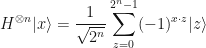
In this blog we are going to explain how we can take a quantum state 


The first thing I want you to notice about the above equation is that we have an 
Where did the 

It clearly went up in to the exponent of the coefficient of
Two things: why did it end up there? And what is the purpose of being able to do this?
To answer the first question: it ended up there because we used some mathematical tricks (which I will explain a little further on); and the purpose? Well, it’s the usual one: we want to change the coordinate system – i.e. we want to change the basis from one which is standard in to one where we want to work in – usually in order to solve a problem that has a clearer or easier representation in the non-standard basis, whatever that is (think: things which are periodic might be better represented in a basis that expresses periodicity as rotations, as a very common example).
Let us now focus on the left-hand side

Do you recall what group we are operating in? Since these are qubits and measurement resolves in to the two-element set 


Thinking about what group you are working in is important because the 0 element is going to be our group (additive) identity – hence the special consideration for this all-zeroes initial state, and for trick #3 below.
But now, going back to the 
Recall that the Hadamard transform generalises to the quantum Fourier transform in
OK, but now let’s do it without the handwaving…
The Bitwise Scalar Product
The first trick we are going to look at to derive the above formula is the following: Suppose we are operating in our cyclic group of integers modulo 2 and we have 


But now suppose we want to know their sum-product; i.e. we want to multiply all their sums, pairwise:

This might seem like an arbitrary request: what is so special about the sum-product? Well, one important application of such a computation is when you calculate the inner product of two vectors.
Now, there is a trick to this, which will help us dramatically in understanding what the Hadamard is doing; and I have to say: in all my reading of Quantum Information and Algorithms I have never seen it derived this way. So hopefully this is a first! Perhaps these tricks are learned in other earlier computer algorithm courses that I never took…
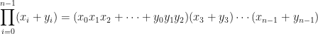
First, we can simply expand the product:

and now let us actually compute the first product:

I want you to count up the number of terms inside the first parentheses: one 


Further, the highest index (subscript) of these terms is 1 (noting that the index runs from 


Now the number of terms inside the first parentheses is 8. This pattern is easy to predict! It should come as no surprise that each time we do this, for each 


where on the right-hand side there are 
Trick #1
Now here is the trick!
These 
Let’s look at some random middle term: 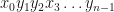
Now that we know what each of the 


Thus we have re-labelled all of the 


Now notice! This indexing runs from
Thus, we have

where a particular
This little exercise should make clear how we go from a product of n terms to a sum of 2n terms. Not only that, we saw how we made a change of basis: we went from
Now let us see if we can apply this trick to the Hadamard transform.
Applying the Trick to the Hadamard Transform
Let the initial qubit register be

where
And now we see why the computational basis is so important here: the Hadamard produces a product of n terms just as before in our example above – except that now the 


Well, almost, the same problem. We already know (from Trick #1) what the answer will look like: it will be a sum of 2n terms. But what do we do about this pesky 
Well, if the number of 

So, from the above trick, we know the answer to this is going to be a sum of 2n terms, so let’s write that down:

and then just quickly insert the negative/positive corrections (inside the interior parentheses):
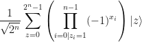
The big product inside the parentheses handles the pesky 

OK, what does this mean now?
This means that for every 
There are only four terms in this case: 


By looking at this simple 
Trick #2
Now we are going to use the fact that in each of these product cases we could have that 

where multiplication here (no operator symbol multiplication) is the element-wise (or pairwise) group multiplication.
In my opinion, this is an interesting way to express this product: the number of instances of the 
Now, using the law of exponents we may write this out in full:

OK, so now we have to be clear that we are in modulo 2, so we write it explicitly.
Trick #3
But now also note that condition on the sum: the 
So we can simply write the sum in the exponent without the condition:
But now we have a breakthrough!
Observe that since the exponent of
…it allows us to make the stunning substitution:
…as required.
Conclusion
There we have it. All the way from the elementary definition of the Hadamard transform, all the way to the generalised Hadmard Transform with no steps skipped and each step clearly defined.
I would say that the only things that need to be done now are to rigorously prove that
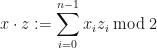
is indeed an actual inner product, and also a little familiarity with how the Hadamard transform generalises up to
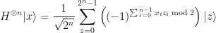
It should now be clear exactly what is going on when you see the formula:

and it is the first example where we start to see the utility of being able to place quantum states (at least their basis – and now remember that the basis is what puts numbers on to abstract things) in to the exponent of the coefficient – a.k.a. in to the phase of a qubit.
This is a very good segway in to another trick called the phase kickback trick which will be the topic of the next blog post in this series. The phase kickback trick is very similar to what is going on in the generalised Hadamard transform with the exception that it sends not a 0 or a 1, but any eigenvalue of any arbitrary operator (i.e. a gate) into the phase.

Very interesting and very cool! I hadn’t yet realized the Hadamard gate could apply to more than two qubits, so this was quite educational.
One question: At the end of Trick #1, the sentence “where a particular x_j is a bit-string of length n.” — should the “x_j” be “z_j”? (If not I may not have understood this as well as I thought I did.)
Thanks Wyrd, yes you’re right. That should be a “z_j”.
This was super helpful, thank you so much! I was learning about the Deutsch-Jozsa algorithm, and I was stuck on on the hadamard transform. Thank you so much 🙂