In the following blog I will be showing you how I installed Octave 6.3.0 for Windows-64 and how I managed to get everything working.
Octave Installation for Windows-64
Install Octave on Windows by going to the https://www.gnu.org/software/octave/download website. I picked Windows-64 (recommended) octave-6.3.0-w64-installer.exe, a 335Mb download.
When it is finished downloading, double-click on the installer executable. Click Next to Continue. Accept the Licence Agreement, and click to install for anyone using this computer. Tick to create desktop shortcuts. If you prefer to use .m file types with Matlab then don’t tick that option. Leave the drop-down box to use OpenBLAS library implementation. Click next.
Leave the default directory and click Install.
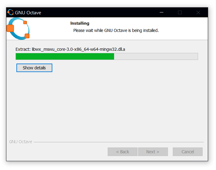
Click Finish and Run GNU Octave.
When you first load up Octave go to the Command Window (if it has not opened by default, then go to Window > Show Command Window).
Like many software programs, Octave uses packages to optionally extend and modify its capability. These packages can be installed and loaded using the built in package management program ‘pkg’. Let us see where the packages are installed by typing in the following:
>> pkg global_listFor me, this returned a path to C:/Program Files/GNU Octave/Octave-6.3.0/mingw64/share/octave/octave_packages, so now I know where my Octave Packages are installed. Note that Octave versions for Windows prior to 6.1.0 defaulted to always making changes to global packages unless the user specified otherwise.
We can list the packages that are already installed by typing in
>> pkg list
Sometimes you may wish to force Octave to refresh its library. You can do this by typing in
>> pkg rebuildThis will force Octave to look for both local and global packages in the set locations to repopulate the list of available packages. Note that ‘local‘ packages always take precedence if the same package is present in both locations.
Package Installation and Update
All packages can be updated to their latest version by running:
>> pkg updateAs this is the first time I have installed Octave on my Windows machine I ran this command straight away.
At first, nothing seemed to be happening. I had the Command Window open so I noticed that I had lost the ‘>>’ command line, so it must be thinking. I waited for a couple of minutes and then I started getting a lot of warning messages.
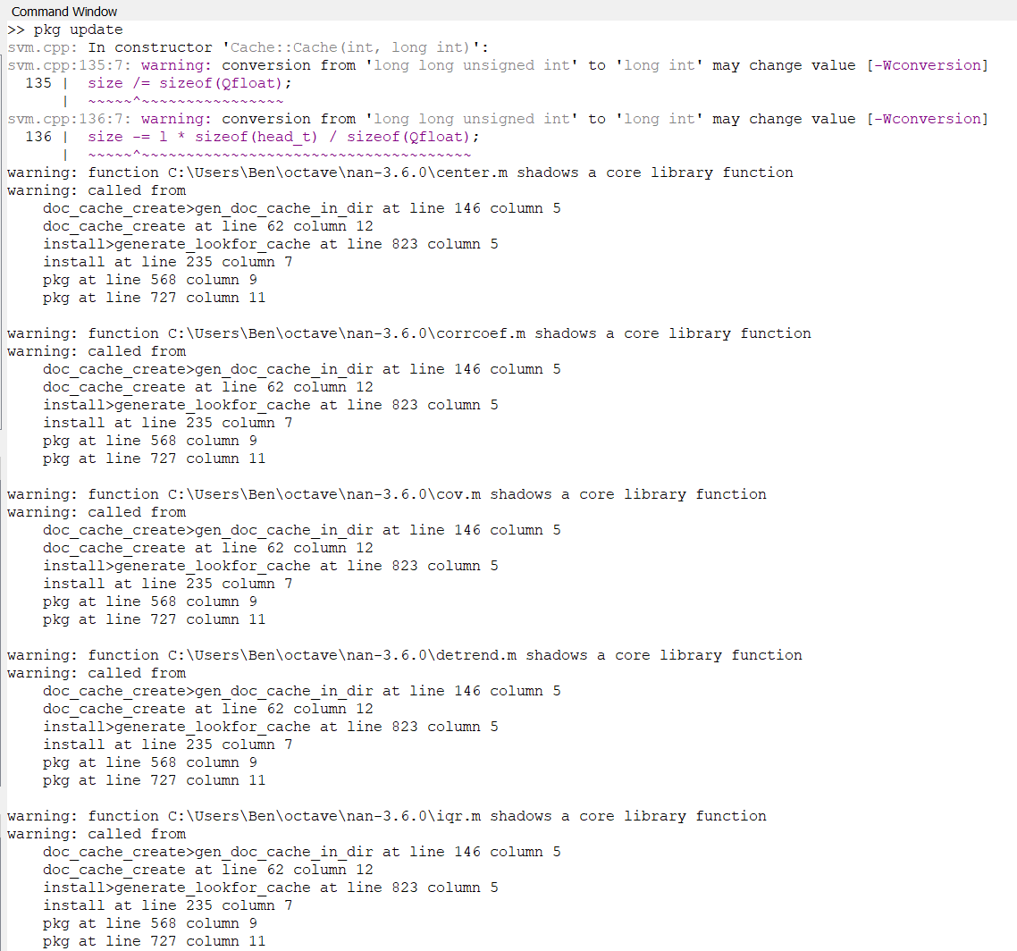
All these warnings seemed to be about doc_cache_create>handle_function at line 98 column 5. I don’t think these are a problem and they seem to be related to the help files in certain library packages.
After another minute of thinking, I had the command line returned to me and all my packages appear to be updated successfully.
The first package I wanted to try to install was the YALMIP package. I read that the way to do this is to run
>> pkg install -forge -local yalmipBut after quickly checking octave.sourceforge.io/packages.php I noticed that this package was not listed there. And sure enough, trying to install the package like this resulted in a ‘package not found‘ error.
Then I went to YALMIP’s GitHub and downloaded the latest official release as YALMIP-master.zip, a 1.3Mb file. I proceeded to unzip the folder, and renamed it to yalmip. Then I copy/pasted the renamed, unzipped folder in to my Octave’s global package folder.
Next, I ran ‘pkg_list‘ to see if the package showed up. I didn’t. So I executed the following command to see if I could force Octave to recognise the YALMIP package:
>> pkg rebuildNope, still not recognised.
Next I tried to navigate to the folder where the zip file is located, using Octave’s File Browser, and right clicked on the YALMIP zip file parent folder and set current directory. Typing in
>> pwdalso confirms what the current working directory is. With the working directory set, I tried to install the zip file as a package:
>> pkg install YALMIP-master.zipbut this resulted in yet another error; this time the package is missing file: COPYING error. I think that the pkg install command expects a tar.gz file.
Adding the Yalmip Directory to PATH
After trying out various install tactics, I ended up noticing that the global variable ‘pwd‘ appeared to hold my YALMIP-master.zip parent directory. So I tried to add it to Octave’s environment variable PATH using the command:
>> addpath(genpath(pwd))and followed that up with the YALMIP test command:
>> yalmiptestVoila! Something appeared to be happening…
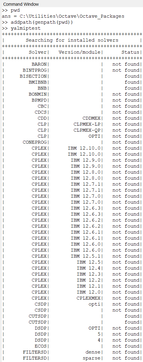
So this looks like it is checking for Solvers; and apparently it has found several calling Bisection, BMIBNB, BNB, CUTSDP, GLPK, KKTQP, LSQNONNEG, and REFINER. I have no idea at all what these are, but at least YALMIP is finally doing something!
The Yalmip Test asked my to press any key to continue the test. I obliged.
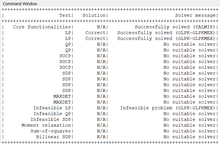
After a few seconds of testing I was given the following command line output:
Creating a sdpvar Variable
One of the objects I really wanted to try out was the so-called Symbolic Decision Variable or sdpvar. Coming from MATLAB myself, I was keen to give these variables a try because I read that almost all MATLAB operators can be applied to sdpvar objects.
I just went through all of the examples from the sdpvar github website and found the matrices pretty easy to create on the command line. I watched the workspace panel as these sdpvar class objects were created.
Vectors and Matrices
We can use the square bracket ![\texttt{ [\,] }](https://s0.wp.com/latex.php?latex=%5Ctexttt%7B+%5B%5C%2C%5D+%7D&bg=%23ffffff&fg=%23111111&s=0&c=20201002)
>> a = [1, 2, 3]

a = 1  2  3
and here is a column vector:
>> b = [4; 5; 6]

b = 4
    5
    6
You can append to a vector:
>> c = [a, 4]

c = 1  2  3  4
and you can use the colon to sequentially fill vectors:
>> d = [2:7]

d = 2  3  4  5  6  7
and to explicitly state the increment:
>> e = [3:0.5:5]

e = 3.0000  3.5000  4.0000  4.5000  5.0000
Create an 
>> A = zeros(M, N)Create a
>> B = ones(M, N)Create a 


>> V = linspace(l, u, N)Given a vector, you can use the parentheses to access an element of the vector according to its position:
>> a = [1:1:5]

a = 1  2  3  4  5

>> a(3)

ans = 3
You can scalar-multiply using the asterisk:
>> a * 2

a = 2  4  6  8  10
and you can element-by-element-multiply using the dot-asterisk:
>> b = [1:2:9]

b = 1  3  5  7  9

>> a.*b

ans = 1  6  15  28  45
There is also the exponentiation operator which can be used element-wise on a vector:
>> a.^2

ans = 1  4  9  16  25
You can matrix-multiply two matrices together using the asterisk:
>> A = [1, 2, 3; 4, 5, 6]

A = 1  2  3
    4  5  6

>> B = [1, 0; 0, 2; 1, 2]

B = 1  0
    0  2
    1  2

>> C = A*B

C =  4  10
    10  22
The transpose can be calculated using the apostrophe:
>> T = A'

T = 1  4
    2  5
    3  6
A very important matrix is the identity matrix. Octave generates these matrices using the ‘eye‘ keyword:
>> I = eye(4)

I = 1  0  0  0
    0  1  0  0
    0  0  1  0
    0  0  0  1
The above identity matrix is a special case of a diagonal matrix, which Octave can generate using the ‘diag‘ function:
>> D = diag([4, 3, 2])

D = 4  0  0
    0  3  0
    0  0  2
Plotting
It’s really easy to plot using the Matlab renderer:
>> angles = [0:pi/3:2*pi]

angles = 0  1.0472  2.0944  3.1416  4.1888  5.2360  6.2832

>> y = sin(angles)

y = 0  0.8660  0.8660  0.0000 -0.8660 -0.8660 -0.0000

>> plot(angles, y)
You can add a third string argument to the plot function to add colour and formatting to your plot. Refer to the following table for options:
| Colour | Marker | Line |
| w = white | . = point | – = solid |
| m = magenta | o = circle (the letter ‘o’) | : = dotted |
| c = cyan | x = cross | -. = dashdot |
| r = red | + = plus | — = dashed |
| g = green | * = star | |
| b = blue | s = square | |
| y = yellow | d = diamond | |
| k = black | v, ^, <, > = triangle (down, up, left, right) | |
| p = pentagram | ||
| h = hexagram |
Thus, we could replace the above graph with this one:
>> plot(angles, y, 'ro-')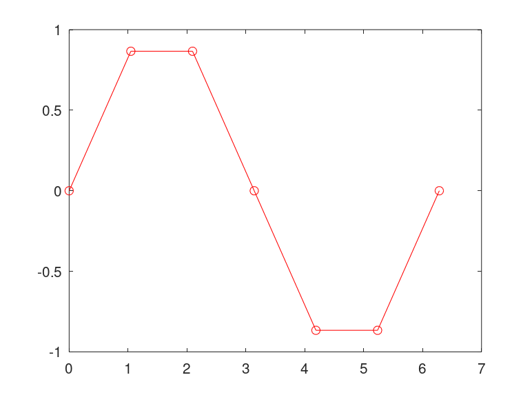
We can add a title and the axis labels in the Editor (note, command line doesn’t work here). Also note that you have to create the plot object first, and then adjust the plot elements like title and axis labels:
plot(angles, y, 'ro:')
title('Graph of y=sin(x)')
xlabel('Angle')
ylabel('y')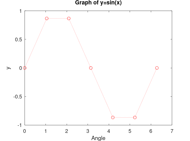

thanks ,i can run yalmiptest after followed your steps.
but yalmiptest run out ,cplex cant found
but i can use cplex (12.8/12.9) in my compute very well
how can i found cplex in my yalmiptest run out?
what is wrong?
but yalmiptest run out ,cplex cant found
but i can use cplex (12.8/12.9) in my compute very well
how can i found cplex in my yalmiptest run out?
what is wrong?