In the previous blog we discussed the Recipe for Pricing. This recipe is a standard way to mix together two stochastic differentials (\textup{d}X_t, \textup{d}Y_t), each with respect to a common source of randomness, say \textup{d}W_t, as a function f(X_t, Y_t), and then to re-write \textup{d}X_t with respect to another source of randomness, say \textup{d}\widetilde{W}_t that carries away any advection (or drift). The point being that under this other source of randomness, the stochastic process has no drift (a.k.a. is a martingale); which makes pricing contingent claims on assets governed by \textup{d}X_t a lot easier, as expectations essentially become percentiles of cumulative normal distributions.

Recap

ARecipeForPricing

As discussed previously, we do this by introducing bias in to the source of the randomness. The bias carries away the drift from the diffusion, and has the equivalent effect of changing the probability measure from, say, a real-world measure \mathbb{P} to a risk-neutral one \mathbb{Q}.

However, to do this we need a degree of freedom. This comes from the mixing of a risky asset with a risk-free asset.

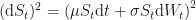
How? Well, here is such a risk-free asset:

\displaystyle M_t := \exp\left(\int_0^t r_s\textup{d}s\right)

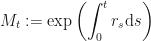
This is the money-market account, or a savings account which earns interest at some non-random (risk-free) interest rate r_t. We invoke the fundamental theorem of asset pricing to ensure that all other assets in the world (say, for example, a stock price S_t) are martingales when priced in terms of this money-market account – that is to say: when S_t is quotiented with M_t, the quotient price S_t / M_t does not drift over time.

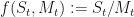
By taking this quotient, we have mixed a risky asset with a risk-free asset, and we can write this operation as a function:

\displaystyle f(S_t, M_t) := S_t / M_t

In the previous article on this subject, we discussed why it is just these two variables (a risky asset, and a risk-free asset) and no others that makes this magic happen; and this does indeed come from the assumptions of the Black-Scholes-Merton (BSM) model that we are working in. In other words, the BSM model describes the evolution of two assets. For example: this savings account M_t earning the risk-free interest rate, and the stock price S_t. Only the stock price asset evolves according to a stochastic driver.

The way in which these two SDE’s are mixed together is three-fold:

  1. through the assumption that we express the risky asset price as a quotient S_t / M_t,
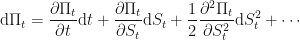
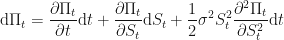
  2. Ito’s lemma – which is a fancy way of expanding SDE’s as a Taylor series, and
  3. by making some assumptions about:
    • how the second partial derivative of time is basically zero,
    • about how Wiener processes square in to time, and
    • about how we include the first and second order terms and can ignore any other terms of higher order.

Ito’s lemma takes a risky \textup{d}S_t and a risk-free \textup{d}M_t stochastic process, mixes them together using Taylor’s Theorem, and outputs a single (Ito) stochastic process \textup{d}f_t, this is this part of the diagram:

ItoLemmaDiagram

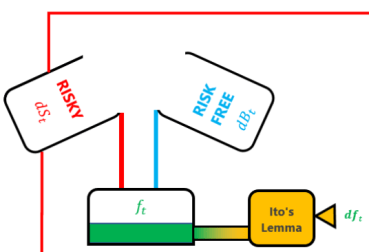
Diagram 1 – Ito’s Lemma produces the \textup{d}f_t stochastic process from a mixing of two processes. This is not the end of the recipe, because we eventually need a driftless version of the \textup{d}S_t process returned.

Next, we take this Ito SDE \textup{d}f_tplus the original real-world probability measure \mathbb{P} and throw this in to Girsanov’s theorem.

GirsanovTheoremDiagram

Diagram 2 – Girsanov’s theorem takes in a Taylor-esque, mixed stochastic process \textup{d}f_t, a real-world probability measure \mathbb{P}, and outputs an equivalent, rigged probability measure \mathbb{Q} and the mixed stochastic process that evolves according to this new measure \textup{d}\tilde{f}_t.

This theorem provides:

  • a brand new SDE \textup{d}\widetilde{f}_t (watch the tilde!),
  • a new probability measure \mathbb{Q}, and
  • an adjusted Wiener process \widetilde{W}_t on \mathbb{Q}.

But there is one major caveat: the new SDE \textup{d}\widetilde{f}_t (with the tilde!) is not necessarily a martingale under the new measure \mathbb{Q}!

That’s right, Girsanov’s theorem only gives you the equivalent measure \mathbb{Q}, not the right martingale to go with it!

But, by making a few algebraic manipulations we can invoke the Martingale Representation Theorem (MRT) to build a third, and final, equivalent SDE \textup{d}f_t (no tilde) so that when written in terms of a Wiener process it  is a martingale under this new measure.

MartingaleRepresentationTheoremDiagram

Diagram 3 – The Martingale Representation Theorem outputs the Wiener differential \textup{d}\widetilde{W}_t and the function f_t from \textup{d}\tilde{f}_t.

This ends the recap. So that in this article we are going to use the recipe again, but this time with a different mixture.

The New Mixture

Recall that last time we mixed a risky asset,

\displaystyle dS_t = \mu_t S_t dt + \sigma_t S_t dW_t

and a risk-free asset,

\displaystyle dB_t = r_t B_t dt

by only extracting the risk-free rate r_t from dB_t and placing it in to the dynamics for a discounted price process,

\displaystyle e^{-\int_0^t r_u du}

to form the mixing equation:

\displaystyle f(S_t,t) := e^{-\int_0^t r_u du}\cdot S_t

This time, however, we will form a linear mixture of the two. I.e., by mixing together \phi_t amount of the risky asset and \psi_t amount of the risk-free asset. We call such a quantity a portfolio and denote it by \Pi_t:

\displaystyle \Pi_t := \phi_t S_t + \psi_t B_t

Let’s stop to think about this for a second.

Why would we want to use the Recipe for Pricing on an additive amount of risky and risk-free positions? Last time, we took the quotient, now we are taking the sum? The quotient allowed us to define the numeraire, but the sum allows us to something else as interesting: the replicating portfolio. We don’t need to know what this is, but it is used in a particular kind of derivation for the fair value of an option on a risky asset in the Black-Scholes framework. We won’t be discussing that here but we will use it as motivation, namely: can we end up with the Black-Scholes partial differential equation using the Recipe for Pricing in the same way?

Let’s get right in to it.

We have our risky asset \textup{d}S_t and our risk-free asset \textup{d}B_t and we have already mixed them additively, giving us a portfolio price process \Pi_t. As usual, we need \textup{d}\Pi_t, so we invoke Taylor’s theorem to get access to those first and second order derivatives:

\displaystyle \textup{d}\Pi_t = \frac{\partial\Pi_t}{\partial t}\textup{d}t + \frac{\partial\Pi_t}{\partial S_t}\textup{d}S_t + \frac{1}{2}\frac{\partial^2\Pi_t}{\partial S_t^2}\textup{d}S_t^2 + \cdots

Let us substitute known quantities because we already know that,

\displaystyle (\textup{d}S_t)^2 = \left(\mu S_t \textup{d}t + \sigma S_t \textup{d}W_t\right)^2

and this simplifies in to

\displaystyle (\textup{d}S_t)^2 = \sigma^2 S_t^2 \textup{d}t

because (\textup{d}t)^{\nu} \rightarrow 0 for all values \nu \geq 2, and (\textup{d}W_t)^2 \rightarrow \textup{d}t.

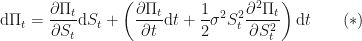
Substituting this in (and truncating the expansion at the second order) we get:

\displaystyle \textup{d}\Pi_t = \frac{\partial\Pi_t}{\partial t}\textup{d}t + \frac{\partial\Pi_t}{\partial S_t}\textup{d}S_t + \frac{1}{2}\sigma^2 S_t^2 \frac{\partial^2\Pi_t}{\partial S_t^2}\textup{d}t

Let us now collect like terms and re-arrange:

\displaystyle \textup{d}\Pi_t = \frac{\partial\Pi_t}{\partial S_t}\textup{d}S_t + \left(\frac{\partial\Pi_t}{\partial t}\textup{d}t + \frac{1}{2}\sigma^2 S_t^2 \frac{\partial^2\Pi_t}{\partial S_t^2}\right)\textup{d}t \quad\quad(\ast)

…and we get stuck.

We cannot proceed any further without making an assumption.

The assumption we want to make is to assume that this portfolio is self-financing i.e. that any purchase of a new asset must be funded by the sale of an old one. There can be no injection of cash or any other funds.

By assuming that this portfolio exists on its own and does not interact with any flow of money we can isolate and pin down the contributors to any infinitesimal change in value of the portfolio.

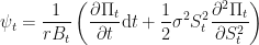
We say that the rate of change of the portfolio value \textup{d}\Pi_t is influenced only by the changes in the values of its constituent positions, namely \phi_t units of the risky asset \textup{d}S_t and  \psi_t units of the risk-free asset \textup{d} B_t.

By making this assumption we actually relieve a degree of freedom from the system, because now the position sizes \phi_t and \psi_t are completely coupled, i.e., to buy more risk \textup{d}S_t (increase \phi_t) we must sell risk-free \textup{d}B_t (decrease \psi_t), and vice versa. The portfolio sum \phi_t + \psi_t remains constant throughout; and knowing \phi_t means to know \psi_t at all times. This relieves a degree of freedom.

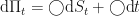
In symbols, this assumption alone allows us to write:

\displaystyle \textup{d}\Pi_t = \phi_t \textup{d}S_t + \psi_t\textup{d}B_t

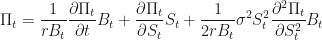
But we already know that \textup{d}B_t = r B_t \textup{d}t, so let us substitute this in to our assumption:

\displaystyle \textup{d}\Pi_t = \phi_t \textup{d}S_t + \psi_t r B_t \textup{d}t \quad\quad(\ast\ast)

Now we have have two equations (\ast) and (\ast\ast) of \textup{d}\Pi_t in the same form, i.e. as a sum of a risky part and a risk-free part: \textup{d}\Pi_t = \bigcirc\textup{d}S_t + \bigcirc\textup{d}t.

So, let us simply equate the terms…

\displaystyle \phi_t = \frac{\partial \Pi_t}{\partial S_t}
\displaystyle \psi_t = \frac{1}{r B_t }\left(\frac{\partial\Pi_t}{\partial t}\textup{d}t + \frac{1}{2}\sigma^2 S_t^2 \frac{\partial^2\Pi_t}{\partial S_t^2}\right)

Now that we have the coefficients, we can substitute these in to the original additive portfolio:

\displaystyle \Pi_t = \phi_t S_t + \psi_t B_t = \frac{\partial \Pi_t}{\partial S_t}S_t + \frac{1}{rB_t}\left(\frac{\partial\Pi_t}{\partial t} + \frac{1}{2}\sigma^2 S_t^2 \frac{\partial^2 \Pi_t}{\partial S_t^2}\right)B_t

Expanding and re-arranging:

\quad\quad\displaystyle \Pi_t = \frac{1}{rB_t}\frac{\partial\Pi_t}{\partial t}B_t + \frac{\partial\Pi_t}{\partial S_t}S_t + \frac{1}{2rB_t}\sigma^2 S_t^2\frac{\partial^2 \Pi_t}{\partial S_t^2}B_t
\displaystyle \Pi_t = \frac{1}{r}\frac{\partial\Pi_t}{\partial t} + S_t\frac{\partial\Pi_t}{\partial S_t} + \frac{1}{2r}\sigma^2 S_t^2\frac{\partial^2 \Pi_t}{\partial S_t^2}
\displaystyle \,\quad\quad\Rightarrow r \Pi_t = \frac{\partial\Pi_t}{\partial t} + r S_t\frac{\partial\Pi_t}{\partial S_t} + \frac{1}{2}\sigma^2 S_t^2\frac{\partial^2 \Pi_t}{\partial S_t^2}
\displaystyle \quad\quad\Rightarrow \frac{\partial\Pi_t}{\partial t} + r S_t\frac{\partial\Pi_t}{\partial S_t} + \frac{1}{2}\sigma^2 S_t^2\frac{\partial^2 \Pi_t}{\partial S_t^2}  - r\Pi_t = 0

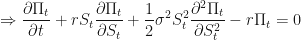
and we are done, because we end up with the Black-Scholes partial differential equation! One can now consult, say Shreve 4.5.14 and easily find solutions to this equation in terms of suitably scaled percentiles of cumulative normal distributions.

Conclusion

We have shown that the Black-Scholes partial differential equation is derivable from the Recipe of Pricing, i.e. through the complicated process of mixing a risky and a risk-free asset together, expanding via Taylor’s theorm, invoking Ito’s Lemma, and then making an assumption about a self-financing portfolio containing a fixed number of positions of varying amounts of the risky and risk-free asset. In this example, note that we did not need to change the measure or invoke Girsanov’s theorem.

Remarkably, two things vanished during this recipe:

  1. The source of randomness \textup{d}W_t vanished during the process of simplifying Taylor’s expansion using the results of Ito, so we did not have to change the measure and find a new martingale. But we did need to make the self-financing assumption about this particular portfolio. This allows the pricing equation to be a deterministic partial differential equation, not a stochastic differential equation.
  2. The risky asset’s drift \mu vanished as well! This means that the Black-Scholes PDE (and solutions of it) do not contain any mention of the drift of the risky asset. This is (and was) a huge deal.

It is remarkable that the value of the self-financing portfolio is completely independent of how fast (or slow) the risky asset grows (or shrinks) in value. The only parameter of the risky asset that remains is it’s volatility.

References

https://quant.stackexchange.com/questions/12788/self-financing-and-black-scholes-merton-formulathis stack exchange question

https://quant.stackexchange.com/questions/8247/why-drifts-are-not-in-the-black-scholes-formula