
We should all be familiar with the Taylor Series (about 


But did you know that this is also just Integration by Parts?
Recall that integration by parts (or IBP) says that
![\displaystyle \begin{aligned}\int_a^b u(y)v'(y)\textup{d}y &= \left[u(y)v(y)\right]_a^b - \int_a^b u'(y)v(y)\textup{d}y \\ &= u(b)v(b) - u(a)v(a) - \int_a^b u'(y)v(y)\textup{d}y\end{aligned}](https://s0.wp.com/latex.php?latex=%5Cdisplaystyle+%5Cbegin%7Baligned%7D%5Cint_a%5Eb+u%28y%29v%27%28y%29%5Ctextup%7Bd%7Dy+%26%3D+%5Cleft%5Bu%28y%29v%28y%29%5Cright%5D_a%5Eb+-+%5Cint_a%5Eb+u%27%28y%29v%28y%29%5Ctextup%7Bd%7Dy+%5C%5C+%26%3D+u%28b%29v%28b%29+-+u%28a%29v%28a%29+-+%5Cint_a%5Eb+u%27%28y%29v%28y%29%5Ctextup%7Bd%7Dy%5Cend%7Baligned%7D&bg=%23ffffff&fg=%23111111&s=0&c=20201002)
Right, so with that in mind, let us generate the left hand side of the above Taylor series. We do this by a trivial application of the main corollary to the Fundamental Theorem of Calculus which states:

So we have our 
The integral can be evaluated by using IBP. Here’s how:
Let 


Now the trick is to set 

Then, by IBPs we have
![\displaystyle\begin{aligned}\int_a^x f'(y)\textup{d}y &= f(a) + \left[-(x-y)f'(y)\right]_a^x - \int_a^x -(x - y)f''(y)\textup{d}y \\ &= f(a) -(x-x)f'(x) + (x-a)f'(a) + \int_a^x (x-y)f''(y)\textup{d}y \\ &= f(a) + \frac{(x-a)}{1!}f'(a) + \int_a^x (x-y)f''(y)\textup{d}y\end{aligned}](https://s0.wp.com/latex.php?latex=%5Cdisplaystyle%5Cbegin%7Baligned%7D%5Cint_a%5Ex+f%27%28y%29%5Ctextup%7Bd%7Dy+%26%3D+f%28a%29+%2B+%5Cleft%5B-%28x-y%29f%27%28y%29%5Cright%5D_a%5Ex+-+%5Cint_a%5Ex+-%28x+-+y%29f%27%27%28y%29%5Ctextup%7Bd%7Dy+%5C%5C+%26%3D+f%28a%29+-%28x-x%29f%27%28x%29+%2B+%28x-a%29f%27%28a%29+%2B+%5Cint_a%5Ex+%28x-y%29f%27%27%28y%29%5Ctextup%7Bd%7Dy+%5C%5C+%26%3D+f%28a%29+%2B+%5Cfrac%7B%28x-a%29%7D%7B1%21%7Df%27%28a%29+%2B+%5Cint_a%5Ex+%28x-y%29f%27%27%28y%29%5Ctextup%7Bd%7Dy%5Cend%7Baligned%7D&bg=%23ffffff&fg=%23111111&s=0&c=20201002)
and we now have the first two terms of the Taylor series!
Continuing in this manner, except now we let

we get:

and it’s hopefully now pretty clear that we could keep going to an accuracy of 

Option Prices
So where do option prices come in to this?
Well, let us first go back to the Taylor series expansion of the function 
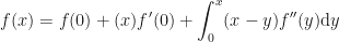
Now we need to do a little bit of geometry to motivate the next trick.
Observe precisely what this 2nd order integral is saying:
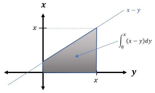
Now let us see what the same integral is over a slightly different function 
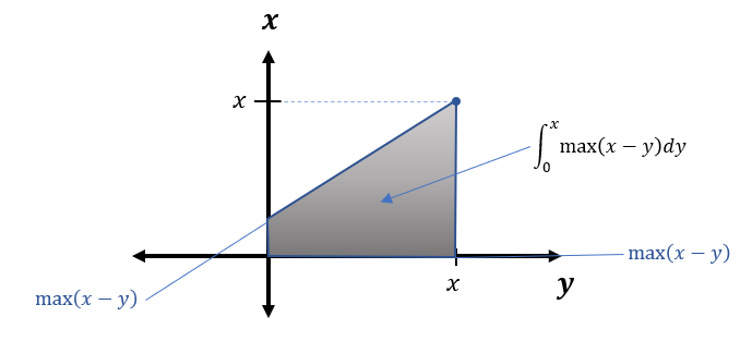
But the trick goes further!
Since we can keep adding 
This means we can write our Taylor series expansion as
This is called writing the series in plus notation.
Let us change notation on the dummy variable 


Note that we cannot jump straight away and say that this integral is the call option price because that expectation (and integral) must be computed with respect to 

But look at what happens when we take the discounted expectation (under the risk-neutral measure) of both sides! In what follows, all expectations are conditional, and taken under the risk-neutral probability measure, i.e. where I will write ![\mathbb{E}[\cdot]](https://s0.wp.com/latex.php?latex=%5Cmathbb%7BE%7D%5B%5Ccdot%5D&bg=%23ffffff&fg=%23111111&s=0&c=20201002)
![\mathbb{E}_t^{\mathbb{Q}}[\cdot | S_t]](https://s0.wp.com/latex.php?latex=%5Cmathbb%7BE%7D_t%5E%7B%5Cmathbb%7BQ%7D%7D%5B%5Ccdot+%7C+S_t%5D&bg=%23ffffff&fg=%23111111&s=0&c=20201002)
First, the left-hand side:
![\displaystyle \textsf{DF}(t,T)\mathbb{E}\left[f(S_T)|S_t\right] =: V(t,T)](https://s0.wp.com/latex.php?latex=%5Cdisplaystyle+%5Ctextsf%7BDF%7D%28t%2CT%29%5Cmathbb%7BE%7D%5Cleft%5Bf%28S_T%29%7CS_t%5Cright%5D+%3D%3A+V%28t%2CT%29&bg=%23ffffff&fg=%23111111&s=0&c=20201002)
This is just the net present value of an option 


Second, the right-hand side:
![\displaystyle \textsf{DF}(t,T)\mathbb{E}[f(0)] + \textsf{DF}(t,T)\mathbb{E}[\underbrace{S_T}_{\textup{Stock}} f'(0)] + \textsf{DF}(t,T)\mathbb{E}\left[\int_0^{\infty} \underbrace{(S_T-K)^+}_{\textup{Call Payoff}} f''(K)\textup{d}K\right]](https://s0.wp.com/latex.php?latex=%5Cdisplaystyle+%5Ctextsf%7BDF%7D%28t%2CT%29%5Cmathbb%7BE%7D%5Bf%280%29%5D+%2B+%5Ctextsf%7BDF%7D%28t%2CT%29%5Cmathbb%7BE%7D%5B%5Cunderbrace%7BS_T%7D_%7B%5Ctextup%7BStock%7D%7D+f%27%280%29%5D+%2B+%5Ctextsf%7BDF%7D%28t%2CT%29%5Cmathbb%7BE%7D%5Cleft%5B%5Cint_0%5E%7B%5Cinfty%7D+%5Cunderbrace%7B%28S_T-K%29%5E%2B%7D_%7B%5Ctextup%7BCall++Payoff%7D%7D+f%27%27%28K%29%5Ctextup%7Bd%7DK%5Cright%5D&bg=%23ffffff&fg=%23111111&s=0&c=20201002)
where we have used the linearity of the expectation operator to split up the operations in to separate additions.
The expectation of the first term (which is constant) is just the constant 
For the second term, the discounted expected stock price under the risk-neutral expectation is just the current stock price, hence: ![\textsf{DF}(t,T)\mathbb{E}[S_T f'(0)] = S_t f'(0)](https://s0.wp.com/latex.php?latex=%5Ctextsf%7BDF%7D%28t%2CT%29%5Cmathbb%7BE%7D%5BS_T+f%27%280%29%5D+%3D+S_t+f%27%280%29&bg=%23ffffff&fg=%23111111&s=0&c=20201002)
For the final term we actually take the discount factor and the expectation inside the integral:
![\displaystyle\begin{aligned}\textsf{DF}(t,T)\mathbb{E}\left[\int_0^{\infty} (S_T-K)^+ f''(K)\textup{d}K\right] &= \int_0^{\infty}\left[\underbrace{\textsf{DF}(t,T)\mathbb{E}\left[ (S_T-K)^+\right]}_{\textup{Call Price}}\right]f''(K)\textup{d}K \\ &= \int_0^{\infty}C_K(t,T) f''(K)\textup{d}K \end{aligned}](https://s0.wp.com/latex.php?latex=%5Cdisplaystyle%5Cbegin%7Baligned%7D%5Ctextsf%7BDF%7D%28t%2CT%29%5Cmathbb%7BE%7D%5Cleft%5B%5Cint_0%5E%7B%5Cinfty%7D+%28S_T-K%29%5E%2B+f%27%27%28K%29%5Ctextup%7Bd%7DK%5Cright%5D+%26%3D+%5Cint_0%5E%7B%5Cinfty%7D%5Cleft%5B%5Cunderbrace%7B%5Ctextsf%7BDF%7D%28t%2CT%29%5Cmathbb%7BE%7D%5Cleft%5B+%28S_T-K%29%5E%2B%5Cright%5D%7D_%7B%5Ctextup%7BCall+Price%7D%7D%5Cright%5Df%27%27%28K%29%5Ctextup%7Bd%7DK+%5C%5C+%26%3D+%5Cint_0%5E%7B%5Cinfty%7DC_K%28t%2CT%29+f%27%27%28K%29%5Ctextup%7Bd%7DK+%5Cend%7Baligned%7D&bg=%23ffffff&fg=%23111111&s=0&c=20201002)
where 
Putting this all together we have that the value 


What does this mean?
Well, it means that a replicating portfolio (attempting to replicate the value of this arbitrary derivative) will be made up of 

Conclusion
We saw in a previous blog that the set of call prices 


with equality as 
And we say that by the Breeden-Litzenberger result, the value of such a Butterfly is approximately equal to (a suitable scaled) terminal probability density function
Then the Fundamental Theorem of Asset Pricing lets you go from a probability density function to a price of a derivative:

In particular, with knowledge of all call prices 
Call option prices span the space of all possible derivative prices (with payoffs at maturity
So really, a replicating portfolio of an arbitrary derivative such as this, will always be some amount of zero-coupon bonds (where we extract the information required for discounting), some amount of the underlying asset (where we ignore its drift, but the difference between its naturally drifting process and the one which doesn’t dertemines the information required for the change of measure), and finally now, some amount of some (infinite) linear combination of elements (call prices) from the spanning set of all possible derivative prices.
References
- Prof. Stephen Blyth, MIT Open Course Ware, Lecture 18.S096 (2013) – https://www.youtube.com/watch?v=eG_aRPy1KVE&t=1935s&ab_channel=MITOpenCourseWare.

Nice article and Blog! Do you also write about Crypto?
Thanks Martin, sadly I know very little about Crypto.
Excellent article. I had never seen this connection (both between TS and IBP as well as TS and Options) discussed before.
There are a few typos that diminshed (ever so slightly) the pleasure of reading this article (v should become y+c and not t+c and also the trick of setting c = -x and not -y; also the plots of x-y are incorrect)
One claification reqd: For the final term when you took the DF and E inside the integral, is it legit? What makes it so?
Thanks!!