Ever wondered what a butterfly has to do with risk management?

In this article, we will take the reverse approach. We will start with some basic math, and work our way to the butterfly.

The Partial Derivative

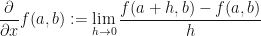
Recall that the (first) partial derivative of a (real-valued) function of two variables f(x,y), with respect to one of the variables, say x, is nothing more than the (first) ordinary derivative of the same function, just with the other variable y held constant. In this context, the symbol x refers to the first slot in the argument list of the function f, while the symbol y refers to the second slot. A concrete example of this two-valued function is when we fix a point, say (a,b) in the space of all possible arguments, which is to say, an (a,b)-coordinate in Euclidean space. Then, the partial derivative of the function with respect to the variable in the first slot (x) is equal to the ordinary derivative (suppressing the second slot), which we then define as gee-prime, or in symbols:

\displaystyle\frac{\partial}{\partial x} f(a,b) = \frac{\textup{d}}{\textup{d}x} g(a) =: g'(a)

In effect, we have fixed the value in the second slot (to which the symbol y points) and we are now varying what we put in to the first slot.

But what is the object on the right-hand side of the above equation?

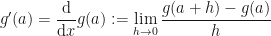
Well, it is simply the derivative of the (real-valued) function of one variable g(x) with respect to x. There is only one slot in the argument list of g, so obviously the symbol x points to this slot.

If the function g(x) traces out a curve in the Euclidean plane, then the derivative of the function traces out a tangent line in the same plane that touches the g(x) curve at the point (a, b) – where b is fixed. So that if we vary the input parameter a, the derivative g'(a) creates a collection of tangent lines – one for each variation of a that we input.

This derivative is geometrically a straight line, so it can be written down as well. Recall the equation of a straight line:

\displaystyle y = mx + b

where m is the gradient of that line, and b is the y-axis intercept. Recall further that the gradient also has an equation: it is equal to the rise divided by the run, as they say. But this is just a fraction:

\displaystyle m := \frac{\textup{rise}}{\textup{run}} = \frac{\Delta y}{\Delta x}

where \Delta y is how far up (or down) the y-axis you rise, and \Delta x is how far right (or left) along the x-axis you run.

Let us re-label the run component of this equation to something a little more traditional: h:= \Delta x. This is the notation you might see in your calculus class.

So h is how far we move along the x-axis whilst traversing the curve specified by g(x). But when we do this traversing, we are also moving a certain amount along the y-axis. Let us say that the amount we move vertically (for a corresponding horizontal move) is the difference of the end point and starting point, that is to say: y_{\textup{end}} - y_{\textup{start}}.

Pretty simply stuff.

So now we have:

\displaystyle m = \frac{\textup{rise}}{\textup{run}} = \frac{\Delta y}{\Delta x} = \frac{y_{\textup{end}} - y_{\textup{start}}}{h}

But since we have already defined the one-variable function g to be one where the second component is fixed, we can use it to measure how far along the y-axis we move. This means that y_{\textup{end}} is equivalent to g(a + h), i.e. given a change in the x-axis by a value of h, the function g(a + h) returns the corresponding change along the y-axis.

So now our gradient equation looks like this:

\displaystyle m = \frac{\textup{rise}}{\textup{run}} = \frac{\Delta y}{\Delta x} = \frac{y_{\textup{end}} - y_{\textup{start}}}{h} = \frac{g(a + h) - g(a)}{h}

Let us say for convenience, that we always just run a distance of 1 unit; so we set h = 1, then the equation y = mx + b describes a straight line with the correct gradient m that passes through the points (x,y) and (x+h,y+g(x+h)).

Wait! This is not a tangent line, because it necessarily intersects the original curve f(x,y) in two places. To make it a tangent, we must decrease our run to zero, i.e. we must have that h \rightarrow 0. This ensures that the line touches the curve at only the one point: precisely at x.

Thus in order for our equation for a straight line to become a tangent line we must introduce this concept of a limit as some variable (e.g. h) approaches zero (written h\rightarrow 0). Indeed, this is the definition of the (first) ordinary derivative:

\displaystyle g'(a) = \frac{\textup{d}}{\textup{d}x}g(a) := \lim_{h\rightarrow 0}\frac{g(a +h) - g(a)}{h}

Now let us re-introduce that fixed, second variable. The ordinary derivative becomes the partial derivative:

\displaystyle \frac{\partial}{\partial x}f(a,b) := \lim_{h\rightarrow 0}\frac{f(a+h,b) - f(a,b)}{h}

and that is as far as we can go without some extra tools.

Taylor’s Theorem

We would like to start discussing the second partial derivative, but we can’t without introducing the very useful tool known as Taylor’s theorem.

Taylor’s theorem says that if a real-valued function g(x) exists and is differentiable at a point x=h (indeed, we have just been using one!) then it (the function) always has an approximation near this point, made up of varying amounts of certain values of the functions: f(x), f'(x), f''(x), etc… In other words, Taylor’s theorem says we can always approximate what the value of the original curve f(x) will be, at any point x = a.

The more values we compute (the more derivatives we perform), the more accurate the approximation gets.

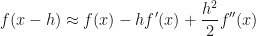
Let us only require second-order approximation, i.e. let us restrict ourselves to computing just the first and second ordinary derivatives. Then Taylor’s theorem says:

 f(x) \approx f(a) + f'(x)(x-a) + \frac{1}{2!}f''(x)(x-a)^2

But recall that the definition of the run was h: = \Delta x = x-a, so upon substitution we get

 f(x) \approx f(x) + hf'(x) + \frac{1}{2!}h^2f''(x)

Let us use Taylor’s theorem twice: once for approximating f(x + h) and a second for approximating f(x -h). We get:

\displaystyle f(x+h) \approx f(x) + hf'(x) + \frac{h^2}{2}f''(x)
\displaystyle f(x-h) \approx f(x) - hf'(x) + \frac{h^2}{2}f''(x)

Adding these two together gives:

\displaystyle f(x+h) + f(x-h) \approx 2f(x) + h^2f''(x)

Rearranging:

\displaystyle f''(x) \approx \frac{f(x+h) - 2f(x) + f(x-h)}{h^2}

And finally, this becomes an equality when we take the limit:

\displaystyle f''(x) = \lim_{h\rightarrow 0}\frac{f(x+h) - 2f(x) + f(x-h)}{h^2}

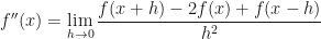
This becomes a partial derivative definition if we re-introduce our fixed, constant second variable:

\displaystyle \frac{\partial^2}{\partial x^2}f(x,y) = \lim_{h\rightarrow 0}\frac{f(x+h,y) - 2f(x,y) + f(x-h,y)}{h^2}

All pretty easy stuff. Right? In fact, already, the answer to our question is staring us in the face. Let us now see how we get from Taylor’s theorem to European option payoffs.

The Partial Derivative as an Option Strategy

Let us now look at this function f(x,y). We have just shown how we can approximate its second partial derivative with respect to the first argument x, and get close to being exact by taking a limit. But take a look at the numerator on the right-hand side of the above equation:

\displaystyle f(x+h,y) - 2f(x,y) + f(x-h,y)

Recall that h:= \Delta x. Let us substitute this back in:

\displaystyle f(x+\Delta x,y) - 2f(x,y) + f(x-\Delta x,y)

Now let us change notation a little to make this next concept clearer. Let us re-label x to be K, y to be T, and re-label the function f to be C. What does it look like now?

\displaystyle C(K+\Delta K,T) - 2C(K,T) + C(K-\Delta K,T)

This is looking like the payoff of four European call options!

In fact it is!

The full approxmation looks like this:

\displaystyle \frac{\partial^2}{\partial K^2}C(K,T) = \lim_{\Delta K\rightarrow 0}\frac{C(K+\Delta K,T) - 2C(K,T) + C(K-\Delta K,T)}{(\Delta K)^2}

This says that the rate of rate of change of the price of an European call option with respect to the fixed, constant strike K (the left-hand side) is equal to a long call option struck at K + \Delta K, a second long call option struck at K - \Delta K, and two short calls struck at K.

Amazing!

In other words, if you had a position consisting of just these four positions, then the portfolio value would be equal to \frac{\partial^2 C}{\partial K^2}.

This specific kind of position is so important and fundamental it carries a special name: it is called a butterfly position.

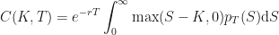
So let us denote the value (at time t) of this butterfly position by B_t. The value, discounted to today (time t = 0) is just B_0 = e^{-rT}B_t, so that:

\displaystyle B_0 = e^{-rT}\left(C(K-\Delta K,T)-2C(K,T)+C(K+\Delta K, T)\right) = e^{-rT}(\Delta K)^2\frac{\partial^2 C}{\partial K^2}

In other words, the value today of a Butterfly is equal to the discounted value of it’s second-order sensitivity to the centered strike K scaled by some fraction of strike, squared.

Butterfly and Second-order Partial Derivative

OK, so we have shown that there is a proportional relationship between the value of a butterfly position B_t and the second-order partial derivative of a European option with respect to strike K.

But wait! This isn’t one of the traditional Greeks. The closest is Delta and Gamma but they are with respect to the underlying asset price S, not the strike K!

Why is this? What can we use this for?

Well, Breeden & Litzenberger showed in 1978 that this partial derivative (and by what we have just showed, also the butterfly position) can be used to approximate the implied (risk-neutral) probability that the underlying asset price S will be equal to the strike K at expiry T.

But can’t you just do the same thing using volatility skew? Well, yes you can, but then you are subjecting yourself to Model Risk. This way, there is no model risk. This is all just supply-demand-arbitrage pricing. In fact, you mix this with the idea that for any time-T (terminal) probability distribution p_T(S), we have the model-free formula for the call price C(K, T) as a function of strike K:

\displaystyle C(K,T) = e^{-rT}\int_0^{\infty} \max(S-K,0)p_T(S)\textup{d}S

The Integral of a Maximum Function

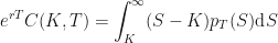
With this knowledge in hand, we can re-arrange to get:

\displaystyle e^{rT}C(K,T) = \int_0^{\infty}\max(S-K,0)p_T(S)\textup{d}S

To evaluate the integral of the maximum function, recall the following little shortcut…

\displaystyle \int_0^{\infty}\max(S-K,0)\textup{d}S = \int_K^{\infty}(S-K)\textup{d}S

…because all values of S less than K contribute nothing to the integral. So we have

\displaystyle e^{rT}C(K,T) = \int_K^{\infty}(S-K)p_T(S)\textup{d}S

Now we need to differentiate both sides with respect to K, noting that the (terminal) probability density p_T(S) does not depend on K, hence it is constant with respect to this differentiation.

\displaystyle e^{rT}\frac{\partial}{\partial K}C(K,T) = \frac{\partial }{\partial K}\int_K^{\infty}(S-K)p_T(S)\textup{d}S

Now, recall the Leibniz Integral Rule, written here for convenience:

\displaystyle \frac{\partial}{\partial x}\left(\int_{a(x)}^{b(x)} f(x,y)\textup{d}y\right) = f(x,b(x))\cdot\frac{\textup{d}}{\textup{d}x}b(x) - f(x,a(x))\cdot\frac{\textup{d}}{\textup{d}x}a(x) + \int_{a(x)}^{b(x)}\frac{\partial}{\partial x}f(x,y)\textup{d}y

And now we make the simple change of variable names: x\rightarrow K, y\rightarrow S, f(x,y) \rightarrow f(K,S), a(x) \rightarrow K, and b(x) \rightarrow \infty. Substituting these in, we get:

\displaystyle \frac{\partial }{\partial K}\int_K^{\infty}(S-K)p_T(S)\textup{d}S = f(K,\infty)p_T(S)\frac{\textup{d}}{\textup{d}K}(\infty) - f(K,K)p_T(S)\frac{\textup{d}}{\textup{d}K}(K)+\int_{K}^{\infty}\frac{\partial }{\partial K}f(K,S)p_T(S)\textup{d}S

Remember, the (terminal) probability density p_T(S) is not a function of strike, so it is treated as a constant here.

Since the derivative is defined in terms of a limit (as we covered initially in this blog), we can treat \frac{\textup{d}}{\textup{d}K}(\infty) = 0. Naively, this derivative is equal to zero no matter how large the number becomes, so we could easily define this as a limit argument: \frac{\textup{d}}{\textup{d}K}(\infty) = \lim_{M\rightarrow\infty}\frac{\textup{d}}{\textup{d}K}(M) = 0. Thus, the first term in the above Leibniz Integral is zero, regardless of how large the underlying asset price S becomes.

The second term in the Leibniz Integral is also zero. This time, it’s because f(K,K) = (K - K) = 0, even though, this time: \frac{\textup{d}}{\textup{d}K}(K) = 1.

This just leaves the third and final term:

\displaystyle\frac{\partial }{\partial K}\int_K^{\infty}(S-K)p_T(S)\textup{d}S = 0 - 0 +\int_{K}^{\infty}\frac{\partial }{\partial K}f(K,S)p_T(S)\textup{d}S

We can evaluate the partial differential under the integral sign (on the right-hand side) as follows:

\displaystyle\frac{\partial }{\partial K}f(K,S)p_T(S)\textup{d}S = \frac{\partial }{\partial K}(S-K)p_T(S)= -\frac{\partial }{\partial K}Sp_T(S) - \frac{\partial }{\partial K}Kp_T(S) = -p_T(S)

Therefore:

\displaystyle e^{rT}\frac{\partial}{\partial K}C(K,T) = -\int_K^{\infty}1\cdot p_T(S)\textup{d}S

Finally, taking the same derivative again with respect to strike K gives:

\displaystyle e^{rT}\frac{\partial^2}{\partial K^2}C(K,T) = -\frac{\partial }{\partial K}\int_K^{\infty}p_T(S)\textup{d}S
\displaystyle \quad\quad = -\left(p_T(\infty) - p_T(K)\right)
\displaystyle \quad\quad = -\left(0 - p_T(K)\right)
\displaystyle \quad\quad = p_T(K)

where the second equality above is given by the 2nd Fundamental Theorem of Calculus, and the third equality is due to the fact that all probability cumulative distribution functions reach 1 at infinity (by definition), and so the probability density there must vanish.

This is known as the Breeden-Litzenberger formula, named after Douglas T. Breeden and Robert H. Litzenberger for their Oct. 1978 paper (published in the Journal of Business, Vol. 51, No. 4, pp 621-651, under Prices of State-Contingent Claims Implicit in Option Prices.

Interpretation

The Breeden-Litzenburger result means that all you need in order to find a (risk-neutral & terminal) probability density p(S,T) is to take the second derivative of various call option prices centered at and around the point you want the density of. The smaller you make \Delta K, the more accurate your estimate of the conditional, terminal probability density at that point becomes!

Indeed, call option prices contain distributional information about the risk-neutral measure \mathbb{Q} (not the real-world, or physical measure \mathbb{P}).

If you have an infinite number of call options at every possible strike, you can determine both the location and the shape of the risk-neutral probability density by calculating the 2nd order partial derivative of the prices w.r.t. the strike. Unfortunately, in order to do this (i.e. to get the price), you would need an implied volatility (or IV) at every point as well. And to calculate the IVs you need the price (using the same formula!).

Indeed, knowing a range of IVs across a range of strikes builds up the volatility smile which, in some way, also reflects the location and shape of the underlying risk-neutral probability density. But if we are to believe Black-Scholes, the underlying risk-neutral density is lognormal, so the IV should be constant across all strikes, and the smile should vanish.

What Breeden & Litzenberger did in 1978 was show how to infer the exact density given knowledge about the call prices and smile across a range of strikes.

Implementation

It is practically impossible to apply the Breeden-Litzenberger result since we cannot make infinitely narrow butterfly spreads, i.e. in practice, h := \Delta x > 0, and so the limiting argument cannot be realised. So we approximate again by interpolating between discrete points.

But where to interpolate?

Naively one might think of performing this interpolation in Price-Strike space, building up the hockey-stick picture. However, it is dangerously easy to accidentally allow arbitrage in to the picture this way. Another nice way to think about it is that since the price of an option is the dependent variable (i.e. the output) of a pricing model which has the usual Black-Scholes inputs: value of the underlying, strike, time to expiration, volatility, and interest rate.

It is much better to interpolate the independent variables (i.e. the inputs) because these should be smoother or better behaved that the output. In the extreme, the moneyness and the time to expiration are so well-behaved, because they are known quantities. In fact, the only degree of freedom that we really have here is the volatility. Which is why it is better to interpolate in the volatility-strike space (or the IV-K space).

I won’t be going in to this part of the implementation here, but allow me to re-direct you to a nice blog on this topic: https://reasonabledeviations.com/2020/10/10/option-implied-pdfs-2. Assuming, however, that we are done, we can convert the IV-K vol curve back to V-K space using the Black-Scholes equation, take the second partial derivative w.r.t. strike (numerically), to find all the points on the probability distribution function using the Breeden-Litzenberger equation.

This generates a butterfly-implied PDF of underlying price movements at maturity time T.

References

Prices of State-Contingent Claims Implicit in Option Prices.

https://reasonabledeviations.com/2020/10/10/option-implied-pdfs-2