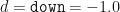
Let us construct a very simple Binomial Tree model with sample trajectories . Each trajectory, for simplicity, will also have time steps, thus time will step from to via steps.
Next, we define our step size for going up and for going down . Let us choose step sizes and . The probability of going up is set to and the probability of going down is set to . This means that at each time step , the price is equally likely to go up as it is to go down. Finally, we will set the initial value to zero: .
Fig 1.1 – Our Binomial Tree Model Parameters
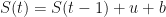
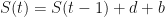
We will also include a (hidden) bias quantity .
Fig 1.2 – Including a (hidden) bias quantity.
The formula governing the dynamics of each trajectory is simple: take the previous value and go up to (with probability ), or go down to (with probability ). Note that each step includes a bias quantity that will become useful later.
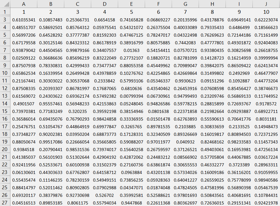
To decide whether goes up or down we will flip a coin. If it is heads, it will go up, but if it is tails it will go down. To implement this in Excel we generate a list of uniformly random numbers between and , then assess, at each time point , if that random number is above or below . Since the random numbers are uniform, this models the randomness of flipping a coin and performing an outcome based on the result. We dedicate a whole sheet in Excel to containing these random ‘coin flips‘:
Fig 2 – An Excel spreadsheet filled with coin flips to help us decide if something is going to go up or down. Time steps run horizontally (10 are pictured), and the random samples run vertically (26 are pictured).
Technically speaking, these are our independent and identically distributed random variables .
To get our first trajectory, we ask at each time step : does . If this is true the we go up: . Otherwise, we go down: .
Fig 3 – Excel Formula that dictates the up and down movement based on the coin flip. Note, the sheet name is “iid”.
where the quantities in the formula are: , and .
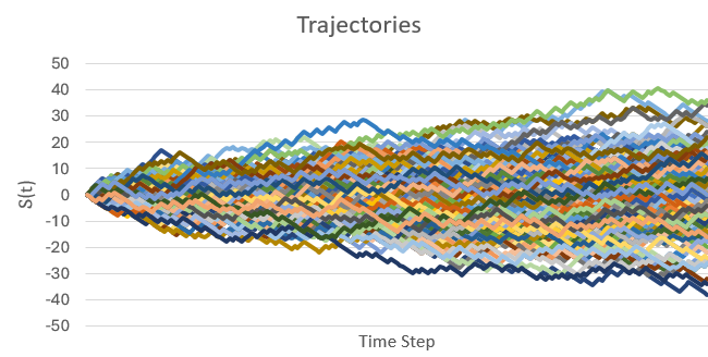
Dragging this formula down by time steps, and then across for trajectories, we get a huge grid of trajectories. Let us plot this grid:
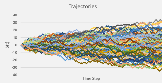
Fig 4 – Plotting all the trajectories with initial value zero, zero bias, and with even chances of moving up or down.
We are showing just trajectories here, which is woefully short of any accuracy that we desire. But accurately predicting trajectories and final positions is not what this article is about. This article is about changing probability measures, and we are about to see how this is done in practice.
Each trajectory will randomly go up and down with equal probability, but this does not mean that it will oscillate around the starting point of . In fact, the odds that a trajectory stays at the whole way along is extremely small, particularly for large numbers of time steps. Some trajectories will end up above zero, while other will end up below zero. The proportion of this split depends entirely on the up probability (and the down probability, since ).
Given enough trajectories, we should expect that roughly half the sample (so ) will end up with a final value and the other half to end up with a final value (ignoring the exactly-equal-to-zero case because, as we said, it’s probability is practically zero).
Now let us focus on the final time , and take the average value, and standard deviation of all trajectory values . In Excel, this is showing as , and . But this means that slightly more trajectories ended up below zero!
If we calculate the sheet again, we get and . Now, slightly more trajectories are ending up above zero.
If we kept recalculating (or equivalently, kept adding more and more sample trajectories), then as this number increases to infinity , the mean should converge to precisely zero (the sample mean), and the standard deviation should be approximatetly equal to the some unbiased estimator of standard deviation.
As said, we are not here to engineer convergence and improve accuracy, we are here to observe how a change in probability measure affects things. However, now that we have an empirical mean and an empirical standard deviation, we have enough to describe a theoretical normal distribution.
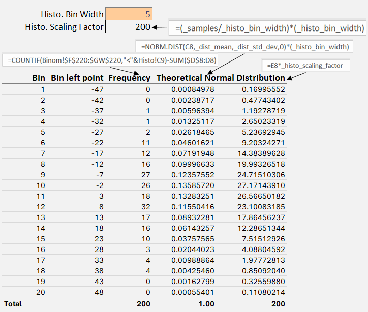
Since normal distributions are completely described by these two parameters, let’s go and create one. Let us again look at the final time slice of all of our trajectories. Now, let us group them in to bins of size . To get the -axis correct, let us query the final time slice for the minimum value and the maximum value, so that our bins contain all the data points.
Fig 5 – Creating the Histogram. The frequency column is a count of the number of trajectories that ended up inside one of the bins. Then we calculate the theoretical percentile of a random number ending up in that bin (i.e. a percentile) using NORM.DIST. The final column on the right is that theoretical number scaled by the number of samples.
Notice that the first theoretical normal distribution defined by the empirical mean and standard derviation does indeed sum to 1. But then, if you want to plot it side-by-side with the empircal frequency histogram you will need to scale it by the scaling factor.
Plotting:
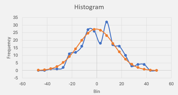
Fig 6 – Plotting the histogram as bin (lower) value by frequency. The blue line shows the empirical frequency of the final value of 200 sample trajectories, which gives a sample mean and standard deviation. The orange line shows the resulting theoretical normal distribution using the sample mean and standard deviation.
Figure 6 shows something interesting. With a probability of moving up and a probability of moving down (step sizes, as long as they are equal in magnitude, are irrelevant), together with a large enough sample size, is enough to make it appear like something is converging toward a normal distribution. We programmed absolutely nothing in to our spreadsheet that should have made the empirical frequency of the final trajectory values gather together like a normal distribution. And yet it does!
Again, we are not here to discuss various things converging, we are here to discuss changing the probability measure – and now we finally get to discuss it.
Changing the Probability Measure
The probability measure that we have been using has been the very simple one:
With no bias (i.e. ) then this particular probability measure results in a very nice, evenly weighted set of trajectories. Notice how they evenly congregate around the starting point zero:
Fig 7 – No bias, and even chance of moving up and down.
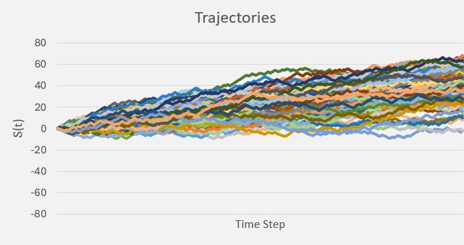
However, let us add a little bit of bias in to the dynamics:
Fig 8 – With a bias of 0.20, the trajectories begin to move upwards more than they move downward. This setting can be achieved by also setting the up value to 1.20 and the down value to -0.80.
We have not touched the probability measure, all we have down is increase the size of the up movement, and decrease the size of the down movement by roughly twenty percent.
Now this is the really important part!
In quantitative finance, the price of a stock, for example, appears to follow such a biased process like the one above in Fig 8. Stocks generally rise over time, and they never fall below zero. Other financial assets behave in a similar way; we say that they all have a property called drift – in this case: they drift upward.
Note that we are neglecting another of their properties relating to jumps, we are assuming no jumps here. I mention this because it is intuitive to think that while a stock price drifts upwards (implying higher up steps that down steps), their down jumps are larger than their up jumps. In any case, a drifting price process is actually rather difficult to deal with (as are processes with jumps, but that’s for another time). Let’s see why.
In quantitative finance, we are interested in the expected value of the price process, denoted , because when the asset we want to price evolves randomly over time, this is our best estimate of the true price. This notation indicates that the expectation is taken under (hence why the probability measure is a superscript) the real-world probability measure – i.e. these are the probabilities that we have attributed to moving up and moving down based on our observations in the real-world.
However, there is not much we can do with this expectation, because an expectation (at heart) is an infinite integral over all on the real line, and so cannot be extracted from the expectation.
Recall from integration methods that the only thing that can be extracted from an integral is a quantity that is constant with respect to the integrating variable. Under the real-world probability measure, the price is definitely not constant. Just look at Fig 8 and tell me that those trajctories (i.e. the ) do not depend on time . If we could remove the drift, then the trajectories do not depend on time, and we would then be able to drastically simplify the expectation by extracting the .
So how do we do this?
What options do we have? Well, we could simply remove the bias. We actually cannot do this, as the bias is part of the observations that we make. The step sizes up and down are the dynamics. If we went and changed those then, yes, we could remove the drift, but then we wouldn’t be looking at the same process anymore.
The only other option we have is to artificially change the probabilities and to something that isn’t fifty-fifty. Yes, we can make this change without affecting the dynamics, because the probabilities represent our collective opinion on the information that we have gathered about the process up to time . So, can we change the probability measure to effectively remove the drift? Yes we can!
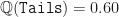
Let us go back to our biased model (Fig 8). Let us now manually change the probabilities and until there is no discernable drift. After playing with a few values of I found that I could effectively remove (in distribution) the drift by setting and
We have changed the probability measure to remove the drift without changing any parameters of the underlying dynamics! The resulting measure is defined as and . By slightly assigning a lower probability to moving up (Heads) and a corresponding higher probability to moving down (Tails), we effectively cancel-out the effect of the observed upward (or positive) drift in the process.
Now, notice some technical things. The new probability measure was found by brute force – i.e. we tested several different measures until we found the one that removed the drift. There is actually a better way to do this that we will discuss in a minute. Also notice that there aren’t any discontinuities: i.e. we don’t suddenly have , where before . Suddenly saying that an event is impossible, where it was possible before, is a bad thing to have in probability theory (it’s very hard to re-normalise probabilities by dividing by zero!). Our change of measure in this case, obviously did not have this issue.
We have thus found in an equivalent measure of , and we write this condition as: . In other words, they both agree on which events are impossible (have measure zero).
So, we have seen that we can convert a drifting process (like the observations of stocks in the real-world) in to one without drift by simply changing the probability measure in to an equivalent one that yields no drift, without touching the parameters of the underlying process. With such a driftless process something really interesting happens to its expectation.
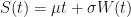
First we assume that the process follows some process, say, the simple arithmetic process defined by , where is that drift we could see (but could not touch!), and where is a Wiener process, which is basically those iid values we generated using a random number generator. This basically implements our trajectories as we had them before.
Substituting directly in to the expectation, we get
Now look at the right-hand side: only when . This equation only has a solution when , i.e. a vanishing drift. Therefore, for arithmetic Brownian motion, only when its drift completely vanishes (say by a probability measure change!) does it yield the very useful property:
i.e. the whole process can be extracted completely from the expectation operator. And if the expected value represents the price of an asset, for example, then now we have a single, real value for it (instead of distribution of possible values).
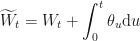
This means that in terms of the infinite integral inside the expectation operator, the process is constant in time, implying that its expectation is constant (so long as we do not look in to the future! this is why these are conditional expectations on the filtration of known information up to time , a small but very important technical condition).
But as we saw before, under . Only under the equivalent measure did the drift vanish!
So how do we go from to being able to write something like ? That circle symbol inside the expectation is basically our manual, trial-and-error, method of trying different probabilities for the up and down movements. Is there an easier way to write this?
We can instead, calculate the Radon-Nikodym derivative. This quantity expresses immediately the correct relationship between two probability measures. The RN derivative is given by
So what is ?
Well, it is precisely the formula that perfectly re-scales all the real-world probabilities under . Theoretically, it has some obtuse form (which we can neglect), but when we use it in conjunction with Girsanov’s theorem, we can skip the direct calculation.
Instead, it tells us that the change of measure can instead manifest as changing the random numbers:
This means that there is a third thing we could have done to eliminate the drift. We could have actually altered the iid random numbers so that the effective ‘coin flip‘ was more likely to be than . But really, this is exactly the same thing. A coin that has been engineered to end up one way over another is exactly the same as changing the probability measure of those results; it’s just two sides of the same equation.
So what the Radon-Nikodym theorem and Girsanov’s theorem tells us is that instead of blindly changing the probability measures until we see the drift disappear, we can just alter the Wiener increments! We just need to know what is.
The value is called the market price of risk and it will have a different formula for different market models. For the arithmetic Brownian motion, it has the formula:
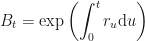
where is the constant drift associated with the risk-free asset ; and by risk-free we mean that it’s price process follows a deterministic one, i.e.
or equivalently
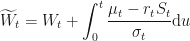
…so we know exactly how to bias our iid numbers (i.e. our Wiener increments) so as to kill off any drift:
This change to how those increments are generated has the exact same effect as manually changing the probability measures from (where ) to (where and ). Now, we don’t need to actually integrate the MPR, it just cancels out the drift term when it’s is substituted.
In this context, the risk-free asset , as defined above, is called the numeraire. And the reason the integral of the MPR cancels out, is precisely because if you take the numeraire, and divide the real asset and form the quotient process then, Ito’s Formula gives the dynamics as in terms of . And this always works for quotient process combined with Ito’s formula this way.
Therefore, the expectation of the quotient process under the probability meaure has no drift and constant expectation in time:
as required.
Conclusion
We have seen that there are three things we can do to cancel out the drift:
Directly change the dynamics (what’s the point?),
Manually change the probability measures until the drift disappears, or
Use the Radon-Nikodym theorem together with Girsanov’s theorem to alter the iid Wiener increments.
The third method is the easiest way, but it completely depends on the model you are using and also the process’s dynamics. As we have seen, under a simple arithmetic Brownian model, using the risk-free money-market bank account as numeraire, we arrive at a nice, clean formula for how we should alter the iid increments. But we also saw, that this eliminates the drift only when we consider the quotient process defined by the original process divided (at each time step) by the numeraire. This quotient process then becomes driftless, and the expectation becomes unique and deterministic in time.


![\mathbb{E}_t^{\mathbb{P}}[S(t)]](https://s0.wp.com/latex.php?latex=%5Cmathbb%7BE%7D_t%5E%7B%5Cmathbb%7BP%7D%7D%5BS%28t%29%5D&bg=%23ffffff&fg=%23111111&s=0&c=20201002)


![\displaystyle\mathbb{E}_t^{\mathbb{P}}[S_t|\mathcal{F}_s] = \mathbb{E}^{\mathbb{P}}[\mu t + \sigma W_t|\mathcal{F}_s] = \mu t + \sigma W_s](https://s0.wp.com/latex.php?latex=%5Cdisplaystyle%5Cmathbb%7BE%7D_t%5E%7B%5Cmathbb%7BP%7D%7D%5BS_t%7C%5Cmathcal%7BF%7D_s%5D+%3D+%5Cmathbb%7BE%7D%5E%7B%5Cmathbb%7BP%7D%7D%5B%5Cmu+t+%2B+%5Csigma+W_t%7C%5Cmathcal%7BF%7D_s%5D+%3D+%5Cmu+t+%2B+%5Csigma+W_s&bg=%23ffffff&fg=%23111111&s=0&c=20201002)


![\displaystyle\mathbb{E}_t^{\mathbb{P}}[S_t|\mathcal{F}_s] = X_s](https://s0.wp.com/latex.php?latex=%5Cdisplaystyle%5Cmathbb%7BE%7D_t%5E%7B%5Cmathbb%7BP%7D%7D%5BS_t%7C%5Cmathcal%7BF%7D_s%5D+%3D+X_s&bg=%23ffffff&fg=%23111111&s=0&c=20201002)


![\mathbb{E}_t^{\mathbb{P}}[S_t|\mathcal{F}_s]](https://s0.wp.com/latex.php?latex=%5Cmathbb%7BE%7D_t%5E%7B%5Cmathbb%7BP%7D%7D%5BS_t%7C%5Cmathcal%7BF%7D_s%5D&bg=%23ffffff&fg=%23111111&s=0&c=20201002)
![\mathbb{E}_t^{\mathbb{Q}}[ \bigcirc| \mathcal{F}_s ]](https://s0.wp.com/latex.php?latex=%5Cmathbb%7BE%7D_t%5E%7B%5Cmathbb%7BQ%7D%7D%5B+%5Cbigcirc%7C+%5Cmathcal%7BF%7D_s+%5D&bg=%23ffffff&fg=%23111111&s=0&c=20201002)


![\displaystyle\mathbb{E}_t^{\mathbb{Q}}\left[\left.\frac{S_t}{B_t}\right|\mathcal{F}_s\right] = \frac{1}{N_t}S_t](https://s0.wp.com/latex.php?latex=%5Cdisplaystyle%5Cmathbb%7BE%7D_t%5E%7B%5Cmathbb%7BQ%7D%7D%5Cleft%5B%5Cleft.%5Cfrac%7BS_t%7D%7BB_t%7D%5Cright%7C%5Cmathcal%7BF%7D_s%5Cright%5D+%3D+%5Cfrac%7B1%7D%7BN_t%7DS_t&bg=%23ffffff&fg=%23111111&s=0&c=20201002)
