In this article we are going to show that starting with a linear algebra picture of quantum computation, we can end up with a dynamic picture of quantum computation that involves a Hamiltonian.
Initally, these two topics may seem difficult to reconcile. Linear algebra is about vectors, lengths or vectors, angles, distances and matrices. This is the basis for classical mechanics. Hamiltonian mechanics, however, is different: It’s all about describing the energy of a system.
We will see that there are but a few relatively simple steps to move from one setting to the other. The insights gained from this transformation will prove extremely useful and by the end of the article I hope you will be comfortable with the Hamiltonian view of quantum algorithms.
What we Already Know
Hopefully your are familiar with matrices. These are the central object of study in linear algebra. We will focus our attention on square matrices – those with an equal number of rows and columns, like this one:
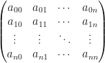
In this case, the size of a square matrix is just the number of rows (or columns) and is denoted by  . Let us also denote such a square matrix of size by the letter
  . We also say that is an element of the square matrices of dimension with complex entries:

When is large it is well-known that matrix inversion (basically matrix division) and multiplication becomes quite difficult. However, it does help if is sparse. All this means is that most of the elements of the matrix are zero – with the standard (although not official) definition being that the number of zeroes is greater than or equal to . Having mostly zero entries in the matrix helps the algorithms that inverts it.
The Fundamental Problem
Let us now introduce the fundamental problem.
Consider the simplest linear interaction of a known Hermitian matrix (we know all the entries of this matrix) with an unknown vector  (we know nothing about the entries of this vector). But now suppose we know the result of this interaction: i.e. we know about a vector
  . Since we have assumed linearity, this interaction can be written down as a mathematical equation:

Our aim is to find which solves this equation. This is our fundamental problem.
Finding is easy when is invertible, because then there exists another  matrix, called
  (with the property that
  ) which solves the above equation. This is because simple rearrangment yields the following equation:

and we are done, i.e. we have alone by itself on the left hand side of the equals sign.
But what if is hard to find? Like in the above case where is large and not sparse?
Then maybe such a direct solution is not efficiently possible. To bypass this issue, maybe instead of trying to find the which solves the problem, we just look for a function of which does. I.e. why not look for an  that solves
  .
.
This is directly translatable in to the world of quantum algorithms because the which solves the linear problem directly, is the quantum state  and this ket is often not even measureable.
Instead, what is measureable (and thus much more useful to us anyway) is the measurement defined by  , which is a function of , rather than just itself. Note that
  is a measurement operator, i.e. it is just another matrix.
When all we need to know is a function of a solution (or equivalently, a matrix operator that acts on ) then it is often acceptable to just know an approximation of that function. This translates to only requiring an approximation of the inverse .
Quick side note: we assumed that is Hermitian (also called self-adjoint) this is to appease the Dirac-von Neumann formulation of quantum mechanics that assumes all physical observables (such as position, momentum, spin, etc…) are represented by these Hermitian matrices). But this also allows for a segue in to the next topic.
Spectral Decomposition
Let us put the fundamental problem aside for a moment and think a little more about the square matrix that we have assumed is Hermitian. Since we are working with Hermitian matrices then always has a powerful property called a spectrum.
When a matrix has a spectrum then it can be expressed as a linear combination.
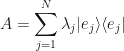
where the  is an orthonormal basis.
It turns out that is more than just an orthonormal basis – it’s an orthonormal eigenbasis, because they all solve the fundamental problem  . Thus, each
  is an eigenvector with eigenvalue
  .
.
Now, off course, in our case each eigenvalue is a real number – the spectrum of a Hermitian matrix is contained within the real line  ; and we can contain the spectrum even further to just the real interval
 ![[-1,1]](https://s0.wp.com/latex.php?latex=%5B-1%2C1%5D&bg=%23ffffff&fg=%23111111&s=0&c=20201002) by forcing the Hermitian matrix to be also Unitary. But more on that later.
by forcing the Hermitian matrix to be also Unitary. But more on that later.
The Hermiticity of , together with the aim to find a solution to the linear equation , gives us this eigenbasis representation.
Eigenvalues, eigenvectors, eigenbasis – these are all special kinds of scalars, vectors and basis vectors that appear when we are talking about any linear transformation on a vector space, and indeed we are, specifically when we talk about the spectrum of a Hermitian matrix. Linear transformations look like our fundamental problem – the attempt to invert the square, Hermitian matrix to find in the linear equation .
So why is all of this so important?
It is important because once a matrix is expressible in terms of a basis of eigenvectors (i.e. an eigenbasis) then it is immediately diagonalizable – and diagonalisble matrices are really powerful. Just look at this example:
Say you have a matrix and you want to compute  . How would you do this quickly when the size of the matrix is huge? It’s very tough actually! Well, don’t run away just yet. What if I told you that was also diagonalisable? Oh, OK. That’s different. If it is diagonalisable then we can find the corresponding diagonal matrix
  by simply computing

where  is invertible and the columns of are just the eigenvectors of , which we already have because can be spectrally decomposed.
Now, instead of manually computing the extremely difficult , we just compute  , and since computing
  is extremely easy (you just raise the numbers on the diagonal without having to worry about any off-diagonal powers), the problem is now really easy – because diagonalisable matrices give you these easily invertible matrices
  for free!
This is why it is so beneficial to us to be assuming we are dealing with Hermitian matrices, because they always have this nice property that they can be decomposed in to their spectrum – that is to say: a linear combination of its eigenbasis – and this allows us to raise these Hermitian matrices to very high powers very easily, regardless of their size .
Being able to raise matrices to high powers is very useful in quantum algorithms because you will be doing a lot of algorithm runs, generating very long sequences of vectors, where you get each subsequent vector by matrix-multiplying the previous one by . But then  , and when
  is large, we make use of the above diagonalisation fact to compute
  .
.
Exponentiation
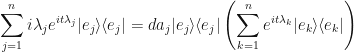
Let us go back to the linear combination representation (the spectrum) of our Hermitian matrix:

Expanding the summation gives:

Since each  is real, we can form this strange-looking object:

This clearly doesn’t equal necessarily, because we’ve exponentiated each eigenbasis coefficient. But the point of this exercise is not to equate such an object with , but rather to say that we can do this, this is a definition – and that this object is actually some other matrix!
So there is this other matrix, call it  , related to (but not equal to it), whose spectral decomposition into the same eigenbasis (we are use the same set of basis vectors here:
  used to represent , is this one whose coefficients are exponentiated.
Now, usually we don’t call this matrix , and although we are free to call it anything we want, we usually denote it by the symbol ` ‘. It’s not really the exponential raised to the imaginary power of – the whole thing is a symbol that pays homage to both the fact that the coefficients are exponentiated, and that the basis of the spectral decomposition is related to .
So we have this object:

If we reverse the spectral decomposition then the symbol still describes an  matrix. But now the elements of this matrix have an imaginary component by virtue of our definition which took the original eigenvalue coefficient
  and exponentiated it to
  . This means, crucially, that we start to have some interesting relationships between the elements of the matrix
  .
.
For example, elements on the left-side of a product (which used to be real for the Hermitian matrix ) are now complex and thus we need to remember the conjugation! This gives multiplication results like:

which holds for all elements where the indices coincide:  . And when the terms are distinct, i.e. when
  , we get full cancellation due to the usual result that
  .
.
This is actually the definition of a unitary matrix! Thus is unitary.
But wait a second…if you think about this for a minute, you’ll realise that this construction always results in a unitary matrix. This is actually the result of a theorem which states that every unitary operator arises as  for some Hermitian operator . Let’s quickly prove this:
Proof
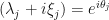
Let

then


hence both  and
and  are real. Now that we know this detail, it implies the following two properties:


Therefore, not only do and have a spectral decomposition (like did above) but they also have ones that share the same basis (like how both and did above). In other words, we can write


which gives us something to decompose  in to:

But since we have already shown that  we must have that each coefficient
  is an eigenvalue of
  , and since is also unitary; and all these eigenvalues have unit norm (a main ingredient we will use in a moment to be able to invoke the geometrical picture of a circle in the plane with radius 1).
It follows from this that each separate eigenvalue and  are real numbers with the property that

Now we have a unit circle! Then for any  , the above equation describes a point somewhere on the circumference of a unit circle.
But now this provides a shortcut!
Because instead of having to keep track of two parameters  for all , we can instead just consider the angle between the line drawn from the point on the circle to the origin and the horizontal. This is always a unique angle (on the unit circle) denoted by
  such that
  and
and  .
.
We thus have
On the left hand side is a unit complex number  with real part
  and imaginary part
  ; and on the right-hand side is the phase of the complex number (note: the magnitude
  ).
).
Now we just reverse the operation of exponentiating that we did in the first place and transform these coefficents like this:  remembering that this is the reverse operation we did initially to do this:
  .
.
This gives us a new spectral decomposition (in the same eigenbasis) with new transformed coefficients:

Q.E.D.
Introducing Dynamics
To introduce some dynamics in to the picture let us define a parameter  whose job it is to track the evolution steps of some algorithm, or just to track time itself. The dynamical evolution of a quantity would be to just let it evolve over and over again, say,
  times so that after that amount of time we end up with
  .
.
This evolved quantity has the same orthonormal eigenbasis  but now with time-scaled eigenvalues
  , which gives a spectral decomposition of

But according to the above proof we have the relationship that this is just a unitary matrix since  , we must have:
  giving:

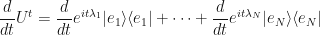
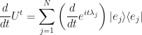
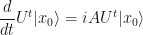
Since this holds for all we can differentiate with respect to time to get
Or, in summation notation:
Now, since we have this additive identity to play with:

…we can insert a bunch of zeroes in to the expansion of  .
.
First, let’s expand the differential again…
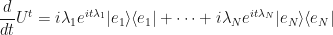
…and then insert a bunch of zeroes:

This might look a little weird but we will make good use of these extra zeroes!
For each zero, insert the identity but just making sure the  ‘s and the ‘s never coincide
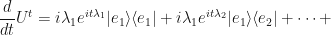
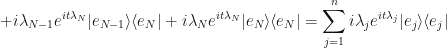
OK, so now we have the same expression, except now we have quite a few more terms which are identically zero, but in their current form allows us to factor out a summation.
Let us try to factor out  from this equation.
Since  we have :
Thus

…our main result for this article!
A quick recap: Start with a Hermitian matrix and consider its spectral decomposition. This will be a linear combination of eigenbasis vectors with eigenvalue coefficients (eigen – because we are assuming we have the linear eigenvector-eigenvalue problem). We then take the coefficients and transform them into  . Undo the decomposition and this forms a new matrix with symbol . This new matrix is unitary, and we now denote it (then we proved this), thus
  . Then we looked at what happened when we multiplied the Hermitian matrix by a real number forming the matrix . This scalar multiplication turns in to exponentiation:
  . Then we differentiated this with respect to and found that time-dependent differential is
 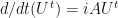 .
.
Using this last fact, let as apply the left-hand side to some initial quantum state ket  . We get
This must hold, since we found that the things operating on the left-hand side of on both sides of the equals sign are the same thing.
But we also know that when  operates on some ket , then this just results in the time-evolution of the ket to a future time state
  . Therefore, the above equation can be simplified to:

If we now define  (because we can! or maybe because some experiment told us to), then substituting this into the above equation and rearranging slightly gives us
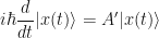
which is precisely the time-dependent Schrodinger equation, where normally one would see  the (observable) Hamiltonian operator, and
  , so that one has instead:
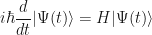
…which is more familiar to us, but identical.
The Schrodinger Equation describes the evolution of an isolated quantum state  in continuous time , but also requires the Planck constant
  to be able to convert between units of time and units of energy (hence why the Planck constant is in units of Joules per Hertz).
Conclusion
Again, this whole derivation is contingent on the eigenvector-eigenvalue problem, i.e. the need to solve the linear equation:

I’ve written a previous article on why this problem is so fundamental. I recommend reading it if this motivation origin does not sit right with you. Before moving on, we noted at this point that it might be more efficient to look for a function of , and gave some reasons for this. As it turns out, the result we get may be interpreted as such, as we will see below.
Then, we needed the first matrix to be Hermitian because we needed all real eigenvalues, and also (probably more importantly) we needed to be diagonalisable. We then exponentiate the Hermitian matrix to form the new matrix . We then saw that this exponentiated Hermitian – which is now Unitary – can be applied to a quantum state and does nothing to it

except for pick up a global phase from it – which is OK because the global phase doesn’t impact measurements.
Since we can write an arbitrary quantum state as a superposition over the (energy) eigenstates

from this perspective, applying the exponentiated Hermitian Unitary gives

and I have seen this described as energy being defined as the speed at which a quantum state picks up a phase – although not obvious to me at this point, but it does sound interesting. The reason why exponentiation helps us so much here is due to a technical result known as Stone’s Theorem (proved by Marshall Stone and John von Neumann in 1932) which is out of scope of this article, but it extremely important and useful.
References
[1] Lipton & Regan, Introduction to Quantum Algorithms via Linear Algebra, 2nd Edition (2021)
[2] Nielsen & Chuang, Quantum Computation and Quantum Information, 10th Anniversary Edtion (2016)
[3] Scott Aaronson’s Lecture Notes (E.g. Lecture 25)

