
Elements of SIMM
What is SIMM?
SIMM stands for Standard Initial Margin Model for non-cleared derivatives.
It is a method for calculating the appropriate level of initial margin (IM) for non-cleared derivatives; where IM is essentially a reserve for potential future exposure (PFE) during a margin period of risk (MPR), capturing funding costs.
Initial Margin is a reserve for potential future exposure (PFE) during a margin period of risk (MPR), capturing funding costs.
Intuitively, IM must be funded as in most cases rehypothecation is forbidden, and we will see how this plays out in a series of illustrations below.
By non-cleared we mean a derivative which is booked with a (third-party) clearing house (like how a listed derivative is booked with an exchange). However, this implies that clearing houses will also implement their own SIMM.
The Global Financial Crisis (GFC) emphasised the precariousness of non-cleared OTC derivatives, particularly with Lehman Brothers and AIG defaulting on many of their contracts.
SIMM was made public by ISDA (the International Swaps & Derivatives Association) in 2013 and the methodology roughly follows seven key principles:
The 6 Guiding Principles
- Shocks are applied to portfolios of derivatives,
- There is some aggregation method,
- A 99% confidence interval,
- A 10-day Time Horizon,
- The use of portfolio sensitivities (greeks) rather than historical simulation and full-reval, and
- The inclusion of a collateral haircut.
I have bolded 5th principle, because the use of greeks to calculate the initial margin is a very interesting one which we will talk about later.
Haircut
A haircut is a discount on the market value of securities taken as collateral. Haircuts can be determined by rules of thumb, negotiation, purpose, or regulatory fixings. Haircuts are put in place by Master Repurchase Agreements (MRAs) for repos, Credit Support Annexes (CSAs) for swaps and derivatives, or by a Clearing Agreements where transactions are exchanged via a Central Counterparty. See the paper written by Wujiang Lou (2017) for more infomation.
The 6 Risk Asset Classes
As with FRTB (The Fundamental Review of the Trading Book) we see instruments being split in to the same 6 asset classes:
- General Interest Rate Risk (GIRR, or simply IR for Interest Rates),
- FX,
- Equities,
- Commodities,
- Credit Spread (Qualifying), and
- Credit Spread (non-Qualifying)
The 5 Buckets
- IR Buckets: based on currency (USD, AUD, EUR, GBP, CAD, etc…)
- FX Buckets: based on each FX pair,
- Equity Buckets: based on sector (Sovereign, Financial, Materials, Utilities, etc…)
- Commodity Buckets: based on commodity (Oil, Gas, Metals, etc…)
- Credit Spread Buckets: based on credit rating (AAA, AA, A, etc…)
The 3 Components of SIMM
Again, as with FRTB, we see that the standard model for SIMM involves the calculation of 3 components:
- Delta Margin
- Vega Margin
- Curvature Margin
The only caveat is that IM for IR and FX is first combined noting a 

Then the Total Portfolio SIMM is equal to the simple sum of everything:

Where Does SIMM Originate?
Economics Without Initial Margin
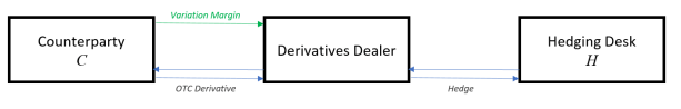
Suppose we are a derivatives dealer. Generally speaking, our OTC (over-the-counter) derivatives position will be with some counterparty 


We represent the OTC Derivative as two arrows between us and the counterparty, for example this could be the cashflows exchanged for an investment in a bond position. There is also the equivalent hedge as two arrows between us and the hedging desk. This might be some fixed-for-float interest rate swap.
As market prices move and up and down, day-to-day, our OTC derivative position could fluctuate into and out of the money. When this position is marked-to-market, depending on who is currently making a profit on this derivative, a variation margin (VM) will be paid. By demanding this margin, derivatives dealers are able to maintain a suitable level of risk which would cover losses experienced by the dealer if the counterparty were to default.
Let’s say that the counterparty has to pay a VM to us. This is typically in the form of a cash payment, but could be any form of collateral. We represent variation margin as a green arrow coming to us:
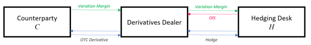
The dealer now cannot simply just sit on a pile of collateral, so they hand it over to the Hedging Desk who can hold on to it, but pays the risk-free rate in return:
The next day two things can happen:
- The Counterparty defaults, and we keep our variation margin to cover the profit that we would have received (remember, counterparty C only pays variation margin if we are currently making a profit on the position), or
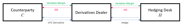
- The Counterparty lives, and, since they loaned collateral to us in the form of the variation margin, will expect some interest payment for that loan.
We consider option 2, and must make an interest payment, usually in the form of some overnight, collateralised interest rate (for example, the OIS rate):
This biggest risk here is the so-called gap risk (or close-out risk).
If the Counterparty defaults then, of course, at that time the dealer has no risk because they are covered by the variation margin (i.e. the Exposure at Default Time is zero). However, default usually takes, on average 10 trading days to play out. In that time, the market could move significantly with us, and the profit that we could have earned in those 10 days would have been lost.
We say that the primary driver for Counterparty Risk (let’s just call it CVA) in this scenario here is the gap risk. However, as explained above, there is very little Funding Risk (FVA).
CVA = Gap Risk
FVA = 0
As we will see, funding risk increases when we introduce initial margin.
Economics With Initial Margin
Now let’s see what happens to our picture when we introduce Initial Margin (IM).
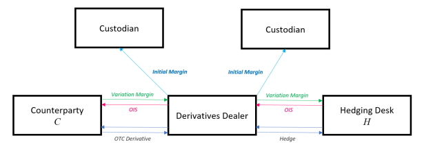
We need to introduce another entity, called the custodian, to whom everyone, including us, pays IM. Initial Margin needs to be paid for every non-cleared derivatives position. Since we have two of these:
- The OTC derivative with Counterparty
- The Hedge with the Hedging Desk
we inevitably pay 2 IMs to the custodian (and we won’t show the IM that the Counterparty and the Hedging Desk also pays):
Now we have 2 outgoing costs. So how does the dealer fund this?
The Dealer will fund the initial margins by borrowing from some short-term Funding Desk 
Now the picture looks like this:
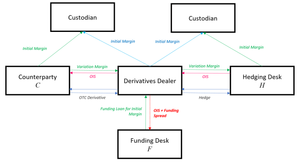
This initial margin being paid by the Counterparty will cover the gap risk in the case of default, which means should the Counterparty default, we will lose practically nothing! Hence, again, CVA is 0, and FVA is also still 0, as in, the Variation Margin is completely funded.
However, we have a new risk (as outlined by the bold red). This is the risk in being able to fund the Initial Margin, we call this MVA.
Uncollateralised, Non-Cleared Derivatives Without IM
If we remove the collateral that the Counterparty posts from the economy then, if they default, we have no compensation. This results in a strong CVA that is roughly equivalent to the Counterparty’s Expected Positive Exposure (or EPE). And since we still have to fund the Variation Margin to the Hedging Desk (Hedging Desks almost always ask for VM when being used to hedge an OTC, non-cleared derivative), we also have a strong FVA that is roughly equivalent to the Counterparty’s Expected Negative Exposure (or ENE).

Uncollateralised, Non-Cleared Derivatives With IM
Under SIMM we still need to post Initial Margin with our Custodian for the Hedge, so this increases the pressure on the funding:

And again, we have CVA roughly equal to the EPE of the Counterparty, FVA roughly equal to the ENE of the Counterparty, but now we have very strong MVA, which is the funding cost of the initial margin that we need to pay to the Custodian.
What is MVA?
In our pictures above, the MVA (the funding risk for initial margin) is roughly proportional to the amount of IM we need to fund.
MVA (margin variation adjustment) is the risk associated with funding initial margin that becomes particularly important when you take away collateral from non-cleared derivatives.
According to ISDA standards, the IM is calculated as a 99% 10-day VaR, hence the MVA is roughly equivalent to the VaR of the Counterparty. This is a very rough, intuitive picture of MVA.
Interestingly, according to Lou, W. (2015) shows that neither Counterparty C or Dealer D can effectuate a true funding cost transfer, unless one side backs down and lets the other side act in a market making role. For accounting purposes, the fair value could remain at the risk-free price, leaving MVA in the bid/ask spread.
He goes on to say that this must be the case when the bilateral trades is settled through a Central Counterparty (CCP). The CCP, as the valuation agent, can’t possibly be aware of either side’s IM funding costs, and the only agreeable valuation it can make is to have the IM cost stripped from the CCP valuation, resulting in the risk-free price.
Calculating SIMM
Since September 2016, the calculation of SIMM for all non-centrally cleared OTC derivatives remains a significant challenge. Especially since IM is a capital measure of potential future exposure based on historical data, it is never-the-less finding its way in to pricing models as MVA.
Green and Kenyon (2015) calculate IM via a Value-at-Risk (VaR) by simulation using a fixed set of exogenously determined historical scenarios, ignoring scenario updating. Brigo and Pallavicini (2014) define IM in the pricing measure, as the 
Technicalities aside, a Derivatives Desk’s primary concern is how to manage trhe transfer of the added cost of posting IM. As outlined above, such an OTC derivative trade does not offer any economic way to transfer the additional cost, unless one party takes the role of a market maker and includes the cost in the bid-ask spread.
Lou (2016) provides an approach to IM as a delta-approximated VaR model, in the pricing measure, that naturally captures the forward scenario updating, with a portfolio-specific multiplier allowing calibration to external models meeting CCP (Central CounterParty) or BCBS requirements.
The methodology used to calculate IM for a given portfolio is often based on historical Monte Carlo (HSVaR), but input parameters in to this model vary significantly between CCPs (e.g. LCH, CME, ICE, Eurex, ASX, etc…)
The Delta-Normal Approximation
Consider the value of a portfolio of derivatives with a common underlying risk factor whose current value is known 


The potential loss of this portfolio would be equivalent to the change in the portfolio value given a 1bp shock of the underlying:
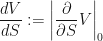
Multiplying both sides by 

But we can substitute
Which says that the potential loss of the portfolio is equivalent to the DV01 multiplied by the normalised change in the underlying.
This is a linear relationship between the DV01 and a change in the underlying, hence the worst loss will be simply experienced when the underlying price changes the most, i.e. an extreme value of

where 

This Delta-Normal VaR is a closed-form solution
Backtesting SIMM
The simplest method is the one defined by Jorion, P. as the failure rate method. This gives the proportion of times VaR is exceeded in a given sample. To arrive at this we simply count the number of times 


Ideally, the failure rate should be an unbiased estimate of the the confidence interval 

However, the number of exceptions should follow a binomial distribution

which we also know has expectation ![\mathbb{E}[x] = pT](https://s0.wp.com/latex.php?latex=%5Cmathbb%7BE%7D%5Bx%5D+%3D+pT&bg=%23ffffff&fg=%23111111&s=0&c=20201002)
![\mathbb{V}[x] = p(1-p)T](https://s0.wp.com/latex.php?latex=%5Cmathbb%7BV%7D%5Bx%5D+%3D+p%281-p%29T&bg=%23ffffff&fg=%23111111&s=0&c=20201002)

The binomial distribution can therefore be used to test whether the number of VaR exceptions is acceptably small.
Netting Sets
A margin set 


A netting set 
For more information about the mathematics of Netting Sets, see Biagini et al. (2019).
The SIMM Sensitivities
For more information, see the youtube video clip here.
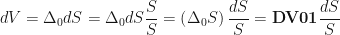
SIMM Vega

SIMM Curvature
where 


See Also
References
- ISDA, “Standard Initial Margin Model (SIMM) for Non-Cleared Derivatives“, (2013)
- Brigo, D., Pallavicini, A., Liu, Q., and Sloth, D., “Non-Linear Valuation under Collateral, Credit Risk and Funding Costs“, (2014)
- Green, A. & Kenyon, C. “MVA: Initial Margin Valuation Adjustment by Replication and Regression“, (2014)
- Lou, W., “Initial Margin Funding Cost Transfer Pricing and MVA“, (2015)
- Lou, W., “Haircutting Non-Cash Collateral“, (2017)
- Zeron, M. & Ruiz, I., “Dynamic Initial Margin via Chebyshev Spectral Decomposition“, (2018)
- Biagini, F., Gnoatto, A. & Oliva, I., “Pricing of Counterparty Risk and Funding with CSA Discounting, Portfolio Effects and Initial Margin“, (2019)

Informative but the text needs to be proofed.
I like the topic and the effort but the computations are not reflecting how SIMM aggregates the risks. You are mixing up product class and risk class.