
In the last article we looked at the quantum Fourier transform (QFT) and how its inverse was used in conjunction with measurement of the output register of entangled qubits to produce the eigenvalues of the applied unitary matrix with probability equal to the absolute value of the amplitude squared. Only a polynomial number of trials was needed to obtain any eigenvalue for which its amplitude was not exponentially small. If the initial guess was close to the desired state then even less trials were needed!
Moreover, once a measurement is made and an eigenvalue determined, the remaining qubits will inevitably collapse in to the state of the corresponding eigenvector. We will see below the intimate relationship with observing an eigenvalue and its corresponding eigenvector. Interestingly, for qubit registers greater than about 40 in size, the state of the corresponding eigenvector already exceeds the entire storage capacity of Google’s Cloud Cluster[3], [4].
What wasn’t really answered was: how does it know what the correct result is?
The short answer is because Abrams & Lloyd figured it out in 1998.
The longer answer is to first consider a much simpler problem:
The Much Simpler Problem to Consider
Let 

where 

When a square matrix has this property then it is called a unitary matrix. A unitary matrix is always a very nice matrix to have. They have several nice properties, several equivalence conditions making them extremely useful for other science applications, plus they are simple enough to be able to model Nature.
So suppose we are given a unitary matrix 


In other words, the matrix multiplication of
This problem is known as the eigenvalue problem and it is a relatively simple problem with a relatively powerful solution. Because that single number has a lot of meaning, if you can find it (not all matrices have eigenvalues).
The way that the eigenvalue problem is posed makes it sound like rotation is bad. Why on Earth would you want to find something that only stretches or shrinks? Firstly, geometrically speaking, stretching and shrinking is equivalent to proportionality – and a lot of powerful physical statements are made on the proviso of proportionality being met (we will meet the proportionality statement that Schrodinger made with his famous equation below).
Also, think of the way you would go about writing down that unitary matrix. Such a matrix is just one way of writing down the components of a linear map in a particular basis (and don’t forget that quantum mechanics and computing is very basis-oriented!). So that matrix will change when you change the basis: a different basis means writing the basis coefficients differently. The eigenvalues do not change – they are invariant under a change of basis!
Eigenvalues do not change under a change of basis.
As a bit of an analogy: it is well-known that every integer can be written as a product of prime numbers – this is known as the fundamental theorem of arithmetic. It is also true that every square matrix can be written as a product of three square matrices 


where 


Unitary matrices have this powerful property that they are always diagonalisable and hence we have the great tool: the eigendecomposition at our disposal to make our calculations of qubit transformations so much easier.
But don’t forget about that vector 
The problem can be reversed too.
You could have instead a unitary matrix 
Take a look at this article for a good, geometric description of what is going on here: https://towardsdatascience.com/eigenvectors-and-eigenvalues-all-you-need-to-know-df92780c591f
Forming Problems
If you have a unitary matrix
which, if solved, forces the vector
In quantum computing we formulate a very similar problem:

See the similarity (pun intended)?
Recall that the state of a qubit has a perfect correspondence with a vector, and the time-evolution (a.k.a. a logic gate application) has a perfect correspondence with a unitary matrix
So what is the eigenvalue
It turns out that it corresponds to the global phase of the qubit. Luckily for us, programming on superconducting quantum computers, our qubits are automatically phase qubits which means we can encode data in to their phases – a trick that regular old classical transistors don’t know how to do. Since, by definition, the global phase of a qubit has no physical consequence on the output state of the qubit we have a direct correspondence with that property and the property of eigenvalues and their impact on eigenvectors. In other words: changes to the global phase does not alter the state of a qubit just as eigenvalues are invariant under a change of basis. I realise this is a bit of a stretch (another pun), but it is still a good analogy in my opinion!
We know exactly how to write down the global phase of a qubit: 
Thus, if we can only interact with a qubit’s global phase, adding to it, subtracting, dividing, factoring it, etc… then we know for sure that we haven’t touched any amplitudes. This is extremely important in quantum mechanics, for two reasons:
- Amplitudes correspond to measurement probabilities, and
- If we change the amplitude we have changed the state of the qubit and we have essentially disturbed it.
Remember, observable quantities (the useful ones!) are directly related to the probabilities of measuring them, which in turn, are directly proportional to amplitudes. A quick and dirty calculation shows this. Take any complex number 

which clearly does not depend on the phase 
Recap
So what have we learned?
We have learned that by framing a problem in a clever way we can force the solution to have a particular desirable property. In the eigenvalue problem, our assumptions in the problem formation itself, forces the solution to have a desirable geometric property, i.e. the vector does not rotate, only stretches or squeezes by an amount equal to
In direct one-to-one correspondence, an equivalent problem can be framed in quantum computing whereby the vector is replaced by the input state vector of a qubit 


The Quantum Problem
So we have a unitary operator 

Our goal is to find
Note that this problem cannot be used to find the solution to just any math problem. It is designed to solve one particular problem – the problem we’ve constructed: an eigenvalue-eigenvector (EE) problem. Which means, you need a unitary matrix, you need and vector. This is not going to solve your financial problems, it is not going to solve how long you will live for, it is not going to calculate the probability that the weather on the weekend will be sunny. Fortunately, the eigenvalue-eigenvector problem is a common problem throughout mathematics and physics, it’s just not applicable everywhere.
The Fourier Transform
One particular problem that the EE-problem solves really well is the Fourier Transform (FT) problem, although this is not immediately obvious.
In the real world, the FT problem seeks to deconstruct a signal (be it audio, radio, X-Ray, light, etc…) in to a small set of fundamental or, I guess you could say, distinguishing frequencies. Similar to the way in which a chord of music can be broken down in to the single keys which make up that chord. I won’t bore you with the detail but take a look at the mathematical form of the Fourier transform:

Keep in mind, this formula was discovered almost 200 years ago and it has the exact same form as our general eigenvalue-eigenvector problem! But already we start to see little pieces of this formula that we’ve seen before. E.g. the 
So is there an equivalent quantum version of the Fourier transform?
Yes there is: the quantum Fourier transform (QFT).
From what we know already, if we just perform our usual substitutions (vector for state vector, unitary matrix for quantum gate, eigenvalue for global phase) we end up with the QFT. In addition, the application of the QFT on a register of qubits will not change the amplitudes and only seeks to add information to the rotation-ness of their global phases. We can see that here in the formula of the QFT:
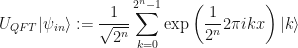
…with just a little abuse of notation because this is the discrete version.
Why Can’t We Do This With Classical Bits?
This is because classical bits can only be in one of two possible states. A bit of information, physically, is usually either a distinct level of voltage or a distinct direction of current. These two definitions of a bit-of-information ruin any chance they have of being qubits – simply because how can you have two voltages simultaneously across a circuit? How can you have two directions of current (ahem, at room temperature) in the same circuit? You just can’t, and so you can’t have these objects simultaneously in two states.
However, some things can! A loop of superconducting metal connected to a Josephson Junction can have two directions of current in the same circuit at the same time! This is known as a phase qubit. Once you have something like that you can write down the electric dynamics as a Lagrangian in terms of the junctions effective mass, the flux, the capacitance (almost said flux-capacitor!), and the gauge-invariant phases differences across the junctions. There will also be a potential energy term in there as well that contains the Josephson energy for the junction along with its critical current.
We then use Josephson’s voltage relations to simplify the Lagrangian and then apply Euler’s equation to find the equations of motion for the phase differences. Using the fact that the bias current must divide the two loops, and using the flux phase relationship one can find the equation for the current flowing through the loop.
Finally, all of this is enough to write down the Hamiltonian of the phase qubit and it turns out (quite amazingly!) that it has the exact same form as the Schrodinger Equation! See the first few pages of Quantum Behavior of the DC SQUID Phase Qubit by Mitra et al (2008).
Indeed, the Schrodinger Equation is also an Eigenvalue-Eigenfunction (EE) problem! As per the definition of an operator, when it acts on a function it produces another function, always, in all cases. However, when it produces something proportional to the original function:

we can always replace proportionality with a constant

Not all functions solve and equation like this, but when it does it is known as an eigenfunction and the proportionality constant is known as the eigenvalue. Quantum mechanics makes the assumption that every experimental measurement is the eigenvalue of some specific (measurement) operator

The eigenvalues 

Summary
In this article I hope I have managed to illustrate just how many physical problems can be reformulated in to some sort of eigenvalue-eigenvector (EE) problem. We see that integer factorisation, Fourier spectral decomposition and even the Schrodinger equation are all concrete examples of the EE-problem.
What is common across all of these problems is the assumption that the thing driving the dynamics is a a unitary operator. We wanted to focus on the Fourier Transform in this setting because in the last article we showed how we could program a register of qubits to perform the same transformation, but it wasn’t exactly clear how the final measurement of those qubits revealed anything about the transformation.
To explain this I tried to convey the idea that algorithms running on qubits are not general purpose, they do not solve arbitrary inputs – they only solve one particular problem, in the case of the quantum Fourier transform, they solve an eigenvalue-eigenvector problem. This is possible because, just as the other analogies we found, there is an equivelent EE-problem here because the Fourier Transform on 
A lot of what has been discussed here was solved by Daniel S. Abrams and Seth Lloyd back in 1998, and if you need further enlightenment on this topic I highly suggest you read this paper. Never-the-less it is interesting to see yet another example of someone, in this case Peter Shor, finding a particular solution to a problem which is just a particular example of a much more general problem that has similar solutions in completely different fields.
References
- Quantum Behavior of the DC SQUID Phase Qubit by Mitra et al (2008)
- A quantum algorithm providing exponential speed increase for finding eigenvalues and eigenvectors, Abrams and Lloyd (1998).
- Quantum supremacy using a programmable superconducting processor, Arute et al., (2019).
- https://www.blog.google/technology/ai/computing-takes-quantum-leap-forward/
