Why Does Shor’s Algorithm Need a QFT? Part I

Measuring the quantum Fourier-transformed state reveals information about the phases of the qubits.

I’ve been wanting to write an article on Shor’s Algorithm (SA) but every time I start I find that I need to devote a large chunk of writing to explaining the Quantum Fourier Transform component, which ends up just taking up way too much of the article.

So instead, I thought I’d write this article to explain, at a high level, why a quantum algorithm would need a QFT in it in the first place; and then tackle Shor’s algorithm in a later article once the groundwork is laid.

Understanding why a QFT is useful in an quantum circuit can lead to a better understanding of the circuit design in general, and this understanding can scale to many other algorithms too.

So we are going to try to get to the point that when you see a “QFT” block in a quantum circuit diagram you won’t have to ask: “why is that there?”.

Shor's_Algorithm — **Figure 1 –** Hopefully, by the end of this article, you will understand why that big $\mathcal{F}^{-1}$ is there. Image courtesy of http://www.wikipedia.com.

**Figure 1 –** Hopefully, by the end of this article, you will understand why that big $\mathcal{F}^{-1}$ is there. Image courtesy of http://www.wikipedia.com.

Introduction

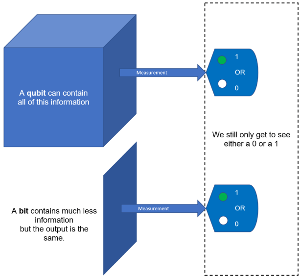
When a register of qubits is entangled and in a superposition, they can contain a huge amount of information, exponentially more than classical bits. The problem is: measuring the register results in the exact same amount of information as would measuring a classical register, i.e. one, single result.

Enter the mighty quantum Fourier transform.

If a problem is framed correctly (and we’ll talk more about that later), then a register of qubits can be transformed in to a new state whereby the measurement of that new state has had all the information focused in to one point with an infinite amplitude.

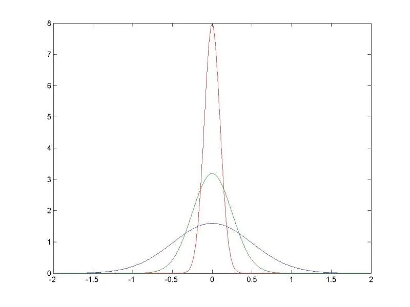
Image result for transform normal distribution to delta function — **Figure 3** – We start with an input register of $2^n$ qubits which are completely entangled and in superposition (the normal distribution). We then attempt to apply a QFT and an inverse QFT to arrive at the peaked distribution which, in the limit, has an infinite amplitude and thus can be interpreted as have a *sure* result. This is a very general idea to what is happening here.

**Figure 3** – We start with an input register of $2^n$ qubits which are completely entangled and in superposition (the normal distribution). We then attempt to apply a QFT and an inverse QFT to arrive at the peaked distribution which, in the limit, has an infinite amplitude and thus can be interpreted as have a *sure* result. This is a very general idea to what is happening here.

We also want to keep in the back of our mind the number one application of this process: Shor’s Algorithm.

Briefly, Shor’s Algorithm (SA) finds an integer’s prime factors. For example, the integer $N = 34866$ can be written as $34866 = 2 \times 3 \times 3 \times 13 \times 149$ where each $\left\{2,3,13,149\right\}$ are prime. More precisely, SA finds the order of an element $a$ modulo $N$ . And so, the problem of finding a non-trivial prime factor of an integer is reduced to finding the order of a non-trivial prime element of the multiplicative quotient group $(\mathbb{Z}/n\mathbb{Z})^{\times}$ .

If that’s too high-brow for you, don’t worry, we’ll get to this in the next article. First, we need to know what QFT can do for us and only then will we start to realise how it can be useful in the problem of finding prime factors.

The General Idea Behind Using QFTs in Quantum Algorithms

In general, you will use a QFT in a quantum algorithm when you have already used superposition and entanglement to encode a problem on to an array of qubits, and now you want to measure those qubits to obtain an answer to your (well-stated) problem.

The problem with measuring a register of entangled qubits in superposition is that you will only ever get one single result (destroying the others) with only some probability that it is the correct one (as per Figure 2).

Instead, if you could somehow transform the register of entangled qubits in to another state altogether that, not only singles-out the correct result but also gives the associated probability of the singled-out result being correct (including the constraint that the sum of all probabilities equal one), then that would be marvelous!

But does such a transformation exist?

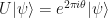
Yes, and it has a name: quantum phase estimation, and the trick is to express the problem as a unitary operator $U$ that acts on the register of qubits such that we have an eigenvalue problem (we covered this here in a previous blog post)

$\displaystyle U|\psi\rangle = e^{2 \pi i \theta}|\psi\rangle$

where $0 \leq \theta < 1$ is knows as the phase.

What is going on in this equation? This says that when you hit the qubit register with this operation you do nothing to it apart from slightly changing its phase.

We also assume that the number of qubits is some power of two, i.e. $N = 2^n$ . Then, if we make these assumptions about $U$ , and they are indeed quite strong assumptions, then two very interesting things happen that allows us to single-out correct results:

The First Interesting Thing

You can split additions in the exponent in to multiplications:

$U^{2^n}=U^{2^n + 0 } = U^{2^n+(1-1)}= U^{2^n-1}U=U^{2^n-1}e^{2\pi i \theta}$

Let’s initiate the pattern again…

$\displaystyle U^{2^n} = \cdots = U^{2^n-1}e^{2 \pi i \theta} = U^{2^n-1+0}e^{2 \pi i \theta} = U^{2^n - 1 + (1-1)}e^{2 \pi i \theta} = U^{2^n - 2}e^{2(2 \pi i \theta)}$

And I can just keep doing this all day long…

Doing this $n-1$ more times:

$\displaystyle U^{2^n} = \cdots = U^{2^n - 2^n}e^{2^n(2\pi i \theta)} = U^0e^{2\pi i 2^n \theta} = e^{2\pi i 2^n \theta}$

and we have this interesting little result:

$\displaystyle U^{2^n} = e^{2\pi i 2^n \theta}$

What does this mean?

Well, it means that if we apply $U$ a total of $2^n$ times then $U$ itself vanishes, and just leaves behind a shadow of itself manifested as a phase quantity $e^{2\pi i 2^n \theta}$ . That’s pretty cool. We made $U$ disappear and got left with a shadowy phase rotation!

This means that anywhere we see $2^n$ applications of $U$ , i.e. $U^{2^n}|\psi\rangle$ we can replace it with $e^{2\pi i 2^n \theta}|\psi\rangle$ , something which we will be doing in the following calculation.

Now let’s make this a controlled unitary operation on qubits. All this means is that you apply $U$ on $|\psi_i\rangle$ in the target register only if $U|i\rangle = |1\rangle$ in the control register.

This means we need two registers: one $|0\rangle^{\otimes n}$ and one $|\psi\rangle$ , together denoted $|0\rangle^{\otimes n}|\psi\rangle$ , consisting of $n$ qubits each.

We also need to apply the Hadamard gate to the first register to get them all in to a superposition, so we have:

$\displaystyle \frac{1}{\sqrt{2^n}}\left( |0\rangle + |1\rangle \right)^{\otimes n}|\psi\rangle$

What we are doing now is covered in my blog on combining Hadamard gates with Controlled-NOT gates. So, read up on that first before continuing.

Even though the point of a Hadamard followed immediately by a CNOT is to obtain Bell states for maximally correlated (and hence entangled) states, we won’t be stopping there in this article. In Shor’s algorithm there is a lot more going on!

Second Interesting Thing

After applying $n$ controlled $U$ operations to each of the $n$ qubits in the target register $|\psi\rangle$ (controlled by states of the control register $|0\rangle$ ), the combined state of the control register (remember, after the Hadamard gate has been applied to each qubit) is:

$\displaystyle \frac{1}{\sqrt{2^n}} \underbrace{ \left( |0\rangle + e^{2\pi i 2^{n-1}\theta}|1\rangle\right)}_{\textup{first qubit}} \otimes \cdots \otimes \underbrace{\left(|0\rangle + e^{2\pi i 2^{1}\theta}|1\rangle\right)}_{(n-1)^{\textup{st}}\textup{ qubit}} \otimes \underbrace{\left(|0\rangle + e^{2\pi i 2^{0}\theta}|1\rangle\right)}_{n^{\textup{th}}\textup{ qubit}}$

This is nothing but:

$\displaystyle \frac{1}{\sqrt{2^n}} \sum_{k=0}^{2^n - 1} e^{2\pi i \theta k}|k\rangle$

where $|k\rangle$ is the binary representation of $k$ , i.e. it is the $k^{\textup{th}}$ computational basis (see the previous article here with a more in-depth explanation) But notice that since all the change is in the global phase part of the summation, the target register is essentially (physically) left completely unchanged! I.e. there is still a $|k\rangle$ on the right hand side of this equation. The only thing that has changed is it phase.

Applying the Inverse Quantum Fourier Transform

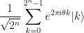
The form of the target qubit register above inspires us to apply the inverse quantum Fourier transform, which yields

$\displaystyle \frac{1}{\sqrt{2^n}} \sum_{x=0}^{2^n - 1} \frac{1}{\sqrt{2^n}} \sum_{k=0}^{2^n - 1} e^{2\pi i \theta k} e^{\frac{-1}{2^n}2\pi i k x} |x\rangle$

which, when you factor out the $1/2^n$ and combine the exponents, equals

$\displaystyle \frac{1}{2^n} \sum_{x=0}^{2^n - 1} \sum_{k=0}^{2^n - 1} \exp\left( -\frac{2\pi i k}{2^n}(x-2^n\theta) \right) |x\rangle$

OK, this still looks a bit complicated, but note that the qubit state is still just a $|x\rangle$ on the right hand side. The physical state has not changed. Just the amplitude has picked up this mighty complicated looking phase! But that’s OK, we know the phase is physically unimportant. Still useful though, definitely useful, because we are packing quite a bit of useful information in there.

Now, we would like to perform a measurement on this second register (as it contains our answers! …somewhere inside that amplitude). However, by definition, quantum measurements must yield real results and therefore are modelled by performing inner products with the measurement state.

Probabilities associated with measurement are then found by taking the absolute value squared, in the usual way:

$\displaystyle \mathbb{P}[a] := \left| \langle a | \psi | x \rangle \right|^2$

Our problem here is that we have no value of $a$ in our expression, we only have $n$ , $k$ , $\theta$ , and $x$ . Uh oh!

How can we get one in there?

Phase Approximation Representation

This is where the phase approximation part comes in!

Take that little exponent part that we have: $-\frac{2\pi i k}{2^n}(x-2^n\theta)$ . Look at that really closely. What have we got?

We know that $\theta \in [0,1]$ is a real number of a closed interval, thus multiplying it by $2^n$ gives $\mathbb{R} \ni 2^n\theta \in [0,2^n]\,\forall n \in \mathbb{Z}$ , which is also a real number, not an integer.

We can always construct a real number as an integer plus an minute difference, i.e. we always have:

$\displaystyle\textup{Real Number } \approx \textup{ Integer } + d$

where $d$ is always less than or equal to one-half, so long as $\textup{Integer}$ is the nearest integer to $2^n$ . Graphically, what we are doing is this:

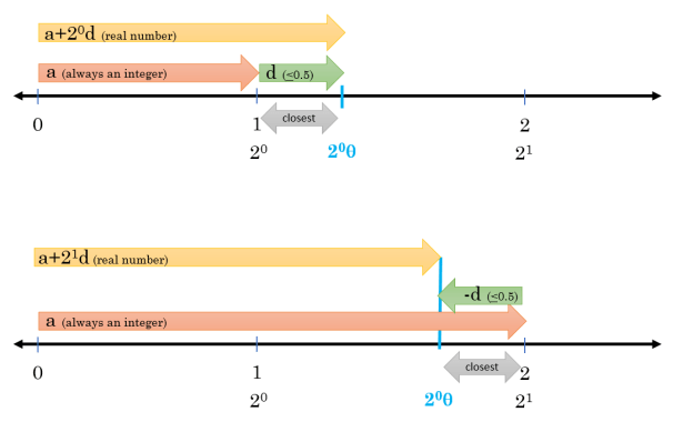
Therefore, we can trash that $2^n\theta$ bit in the exponent, and just approximate it with

$\displaystyle 2^n \theta \approx a + 2^n d$

for all $n$ , where $a$ is the nearest integer to $2^n \theta$ , and the difference (which scales with $n$ ) satisfies the bounds

$\displaystyle 0 \leq |2^n d | \leq \frac{1}{2}$

This approximation does have an integer component $a$ , and that’s how we introduce it! This is Phase Approximation and this is why we do it.

Now we have an expression, with a discretised, approximated phase that includes an $a$ in it we can continue. So, beginning with our state which has been QFT’d and then inverse QFT’d:

$\displaystyle \frac{1}{2^n} \sum_{x=0}^{2^n - 1} \sum_{k=0}^{2^n - 1} \exp\left( -\frac{2\pi i k}{2^n}(x-2^n\theta)\right)$

…we then replace the real number $2^n \theta$ with it’s approximation:

$\displaystyle = \frac{1}{2^n} \sum_{x=0}^{2^n - 1} \sum_{k=0}^{2^n - 1} \exp\left( -\frac{2\pi i k}{2^n}\left(x-(a+2^n d \right)\right)$

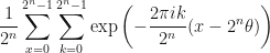
…expand the exponent:

$\displaystyle = \frac{1}{2^n} \sum_{x=0}^{2^n - 1} \sum_{k=0}^{2^n - 1} \exp\left( -\frac{2\pi i kx}{2^n}+\frac{2\pi i k a}{2^n} - \frac{2\pi i k 2^n d}{2^n} \right)$

…and now factor out the common factor of $e^{2\pi i dk }$ to finally get:

$\displaystyle = \frac{1}{2^n} \sum_{x=0}^{2^n - 1} \sum_{k=0}^{2^n - 1} \exp\left( -\frac{2\pi i k}{2^n}(x-a)\right)e^{2\pi i d k }$

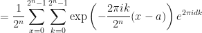
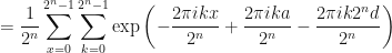
Performing measurement in the computational basis on the first control register yields the result $a$ with probability:

$\displaystyle \mathbb{P}[a] = \left| \left\langle a \Bigg| \frac{1}{2^n} \sum_{x=0}^{2^n - 1} \sum_{k=0}^{2^n - 1} \exp\left( -\frac{2\pi i k}{2^n}(x-a)\right)e^{2\pi i \delta k }\Bigg| x\right\rangle \right|^2$

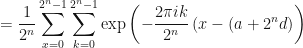
Evaluating the left-hand side of the inner product first, we see that when we substitute $x = a$ , we get $(a-a)=0$ in the exponent. So that part reduces to 1.

We can also pull out the $\frac{1}{2^n}$ outside of the absolute value squared to get $\frac{1}{2^{2n}}$ .

Lastly, since the $(a-a)=0$ cancellation leaves us with no terms with $x$ in them, the $x$ -summation disappears as well, and we are left with:

$\displaystyle \mathbb{P}[a] = \frac{1}{2^{2n}} \left| \sum_{k=0}^{2^n - 1} e^{2\pi i \delta k } \right|^2$

What can we say about this measurement?

When $d = 0$ , which implies that $2^n \theta$ is precisely an integer and no approximation is necessary, then (remember, going from zero to $2^n - 1$ is, in fact, $2^n$ terms!) we get:

$\displaystyle \mathbb{P}[a] = \frac{1}{2^{2n}} \left| \sum_{k=0}^{2^n - 1} e^{2\pi i \delta k } \right|^2 = \frac{1}{2^{2n}} \left| \sum_{k=0}^{2^n - 1} e^0 \right|^2 = \frac{1}{2^{2n}} \left| 2^n \right|^2 = \frac{1}{2^{2n}}(2^n)^2 = \frac{2^{2n}}{2^{2n}} = 1$

In other words, the qubit register, when measured, yields the correct result $a$ with probability 100%.

Wow!

What if $d \neq 0$ ?

Then $2^n\theta$ is not an integer, and the qubit register, when measured, yields the correct result with probability bounded below by 40.5%. Which is a pretty good lower bound, and, in fact, can be increased to practically 100% by including more and more qubits in the register[1].

Summary

So what have we done so far?

Well, we have assumed that our mathematical problem can be expressed as a unitary operator on the input register of $2^n$ qubits. Using the properties of the unitary operator, results from the eigenvalue problem, and the fact that we have exactly $2^n$ number of qubits we found that we could express the unitary operator as an exponential with phase equal to some factor of $2^n$ , in other words, the size of the register becomes part of the phase of the mathematical problem. Then we found that the exponential could be factored in to a product of $n$ factors. (where those factors themselves were motivated by the potential to implement each one as a Hadamard and Rotation gate in a quantum circuit). But then we noticed that the expanded, factored expression is precisely that of the quantum Fourier transform that we found in the previous article here.

Thus, assuming unitarity, eigenvalue proble, power of two sizes of qubit registers, and the factors being Hadamard and Rotation gates, we find that the exponentiated factorisation has precisely the same form as if we had just applied a quantum Fourier transform!

The beauty of this result looking exactly like the quantum Fourier transform is that all the transforming going on is only occurring with the global phases of the qubits, and not with their actual physical components. Thus, if we had encoded a mathematical problem in to a register of qubits, then our assumptions of unitarity, size, and factoring in to $H$ and $R$ -style gates, does not alter the state of the qubit – only their phases. One could say that all the information of the problem is now encoded in to the global phase of the register – which is essentially something we can do as much as we like without destroying the structure of the problem.

To get an actual result, however, we have to transform the information held in the global phase back in to a target register of qubits $|x\rangle$ . To do this we applied the inverse quantum Fourier transform and found that if the phase (which is a real number with modulus) was exactly an integer then the global phase transforms back in to one single result with 100% probability of being measured! This is because the inverse QFT maps the exponentiated factored input register back in to a state that has focused all the amplitudes.

Which is utterly amazing in my opinion.

However, the likelihood that the global phase is exactly an integer is minuscule, practically zero. But the neat thing about this setup is: when the phase is not a integer the global phase transforms back in to one single result with a non-zero probability – not a zero probability as if it were, say, a uniform probability distribution (which is what it is in the beginning). In fact, the probability is dependent on the size of the input qubit register, and repeated measurements will only serve to increase the probability of obtaining a correct answer, theoretically to 100% in the infinite limit.

While we have enforced quite a number of assumptions in this setup, it is still truly remarkable, yet completely mathematically logical, that performing, essentially what is a discrete quantum Fourier transform and then applying the inverse quantum Fourier transform gathers together the amplitudes and focuses them in to a delta-like function right at the point that we need it to. The algorithm knows to do this because that point where all the amplitudes are focused is an eigenvalue of the unitary operator, and we get to build the unitary operator any way we like so that it solves our well-framed problem. Different unitaries will solve different problems.

Therefore, the quantum phase estimation algorithm utilises the power of linear algebra to manipulate the global phases of a register of entangled qubits in superposition such that the inverse quantum Fourier transform provides the answer that we are looking for (of the associated unitary) with an infinite amplitude, a.k.a. 100% surety.

Coming Up

In the next article we will be discussing Shor’s algorithm and how it used the sorcery of quantum phase estimation to find prime factors.

References

[1] Cleve, Ekert, Macchiavello, Mosca – Quantum algorithms revisited, Proceedings of the Royal Society 454 (1998).

[2] Nielsen, N. & Chuang, I. L. – Quantum Computation and Quantum Information, Cambridge University Press, (2010).

	Scarlett Tavores on The Hadamard Transform
	eo on Probability Distributions in…
	benjaminwhiteside on Options Hide in Taylor Se…
	Martin on Options Hide in Taylor Se…
	Veli on What is IRRBB?

From First Principles

Mathematics Without Hand Waving

Why Does Shor’s Algorithm Need a QFT? Part I

Introduction