
In this blog we are going to start working on a brand new Python library; and the first thing which we will be doing is creating probability distribution objects.
Now, scipy.stats does an excellent job at providing such probability distributions as class objects, and we will be leveraging heavily on this python package; however, we will be designing our own (wrapper) classes over the top to satisfy our particular needs.
Distributions
The first Python module we are going to need is one which contains all of our Probability Distributions as Python Objects. So let’s go ahead and open up our PyCharm IDE and create a new Python file and call it distributions.py.
In this file we are going to need numpy and scipy, so we are going to install these Python packages and import them:

They are greyed out because we haven’t written any code yet that uses them! Let us now create the skeleton of an abstract base class for probability distributions:
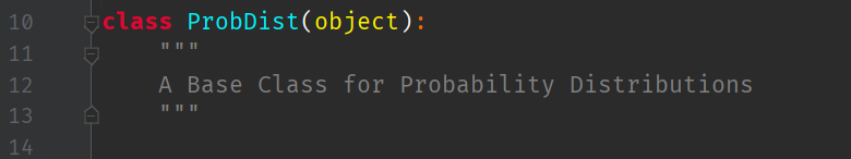
The first method this class will have is the ability for it to return to the user a (univariate) probability density function 

What else can we do?
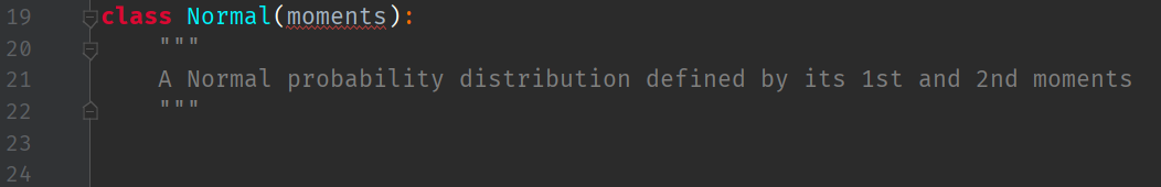
Well, we know that a Normal probability distribution should be defined here as well. All Normal distributions are specified completely by their first and second moments, i.e. by their mean 

We can define a skeleton derived class here like so:
This class will be constructed by passing it a set of parameters 
Sampling
This prompts us to add a new method to the base class: one should have the ability to sample random variables from the distribution!
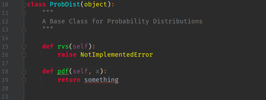
Let us call this class method rvs for “Random Variables“, and implement it in the base class:

Let us defer the implementation of the random variable to the inheriting class by using the keyword: NotImplementedError:
This means the the Normal distribution class will need to implement its own rvs method:
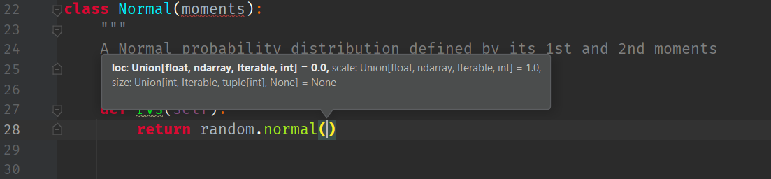
We will use the Numpy Random library to implement the Normal Random Variable method. However, it needs loc (i.e. the first parameter: the mean, 
This means, that the ‘moments‘ argument
But let’s be a little bit more clever than that. Let us define a new class object (called TwoParameterDist) that holds any two, generic parameters called loc and scale:

Now, we can simply initialise the Normal class with the TwoParameterDist class, and refer to any loc or size as TwoParameterDist.loc or TwoParameterDist.scale.
When we instantiate a Normal ProbDist from a TwoParameterDist object, the Normal class inherits loc and size from TwoParameterDist. Thus, we can always access data held in the TwoParameterDist object after instantiating Normal by typing self.loc and self.scale.
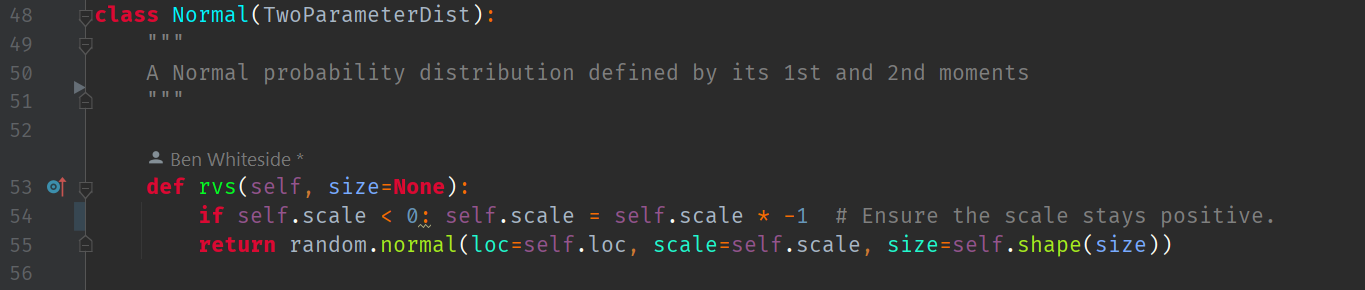
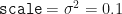
The rvs method of the Normal ProbDist class now returns a numpy random.normal random variable where:
- loc <- mean,
- scale <- variance,
.
The Size of a Probability Distribution
Note that we allow an optional parameter called size to potential reshape the distribution if we need to. The size, in this sense, is the dimensionality of the distribution. For all univariate cases, the size is 1. In later blogs on extending this module we will investigate multi-variate probability distributions where the size is greater than 1.
This allows us to fully use the numpy random normal class. The size (or dimension) parameter is not a moment, so it can’t reside in the TwoParameterDist class. Hence, we place the size further up, in the parent base class ProbDist (i.e. the dimension of a probability distribution is a property of a ProbDist):
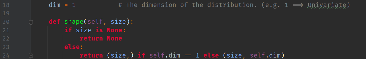
Note that since size() is implemented as a method in the base class, to access the size parameter we must call the method with the parentheses operator. The other two parameters are accessed as public, inherited class data.
The Inverse CDF
Another method we can quickly implement here without additional infrastructure is the percent point function (or inverse CDF) function at a particular quantile 

Testing
Let us now perform a unit test of this implementation.
We create a new Python file called main.py and import our distributions class as dist:
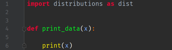
Notice that I have also created a little print function, so I can print the results of calling rvs or ppf to the console.
Next, in the usual fashion, we create a test case:

Line 15 shows us instantiating a new Normal probability distribution class with the initial parameters 
Then, line 17 shows how we then ask the instantiated distribution object for a single random variate 

The random variate we got in this case was 
Structured Distribution
A structured distribution (or 

By a 

Since
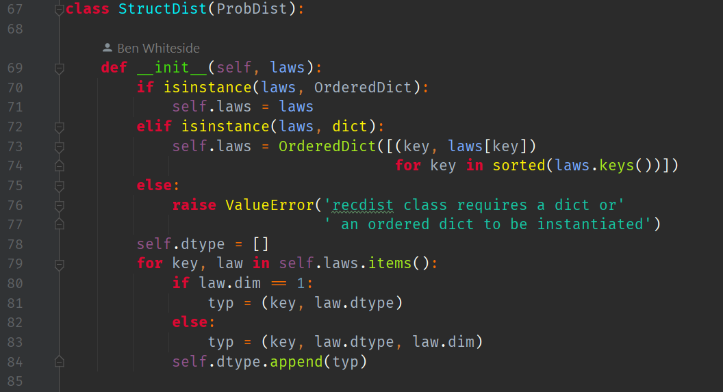
We implement this class to sit between user-defined dictionaries of random variables and their probability distribution functions. This allows the user to specify a random variable label, say 
Note that while the 

After processing, the laws dictionary becomes part of the
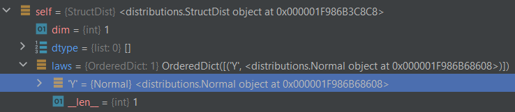
This is a good way to associate a variable name
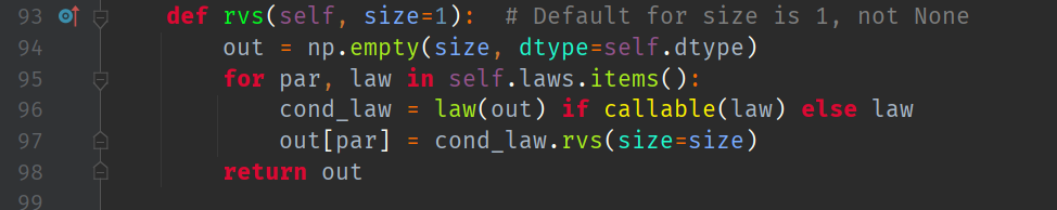
The StructDist class will also need to implement its own rvs method, except this time it is generic. I.e. any time we need a particular probability distribution, we refer to that as a law:
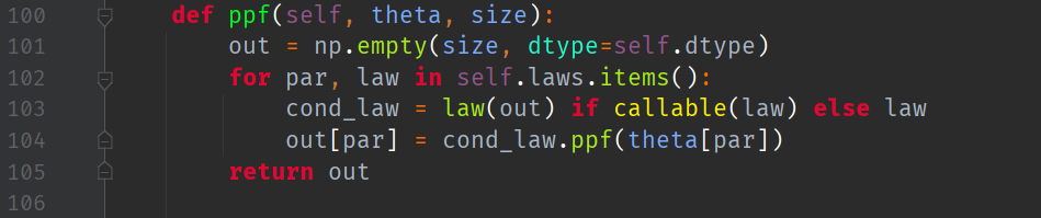
Likewise, for the corresponding implementation of the Inverse CDF method:
Plotting Samples Drawn from Distributions
We instruct Python to make histogram plots of discrete probability distributions via the use of a dictionary. Here, I have labelled my random variable as 

We then instantiate a StructDist with the above ‘law’ dictionary:

Now, we run a test. Let us attempt to sample 5000 random variates
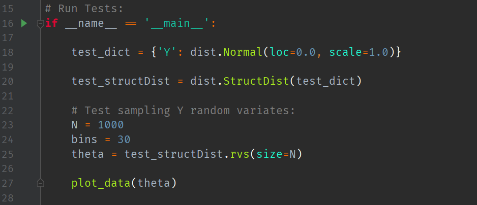
giving the following Seaborn plot:

This uses a custom plot function:
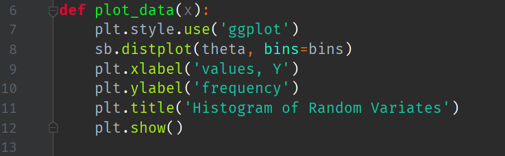
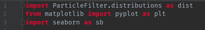
where we have imported the following:
Conclusion
In this blog we have successfully wrapped the scipy.stats normal distribution class in to a custom wrapper class. We also created a new structure of distributions to hold pairs of labels and laws. Then, we showed how easy it is to store such pairs and then sample from them.
In the next blog we will implement a state space model.

Hi! Nice start, where’s the statespace model? 🙂
Hi, nice starting post, where’s the statespace model 😛
Currently working on that blog as we speak! Hopefully it will be published next weekend.
Could you please upload the entire script as like one image? It would be nice to see what you were doing visually. Makes it much easier for us to follow along.