In this blog we are going to continue working with our Dark Mode Jupyter Notebooks which we started in the previous blog linked here.
It’s always good to keep up-to-date with the Qiskit library, and it’s also nice to continually ensure that we can create nice looking, dark-themed Jupyter notebooks for our work with Qiskit, especially the visualisations! So, in this blog, we are going to work through setting up a new Jupyter notebook python environment, install some new Qiskit packages, and see if we can get all the visualisations working in dark mode.
Setup
Assuming that you have Python 3 installed and also installed Anaconda, then open Windows start menu, and search and open Anaconda Terminal.
When Anaconda Terminal loads, type in conda env list to remind yourself of your environments.
Create a new Anaconda Environment from the command line by typing in
conda create -n ENV_QUANTUM python=3It will ask you to confirm that you want to install and update the base python packages for this new environment. Type y to proceed.
Typing conda env list should now show the new environment:
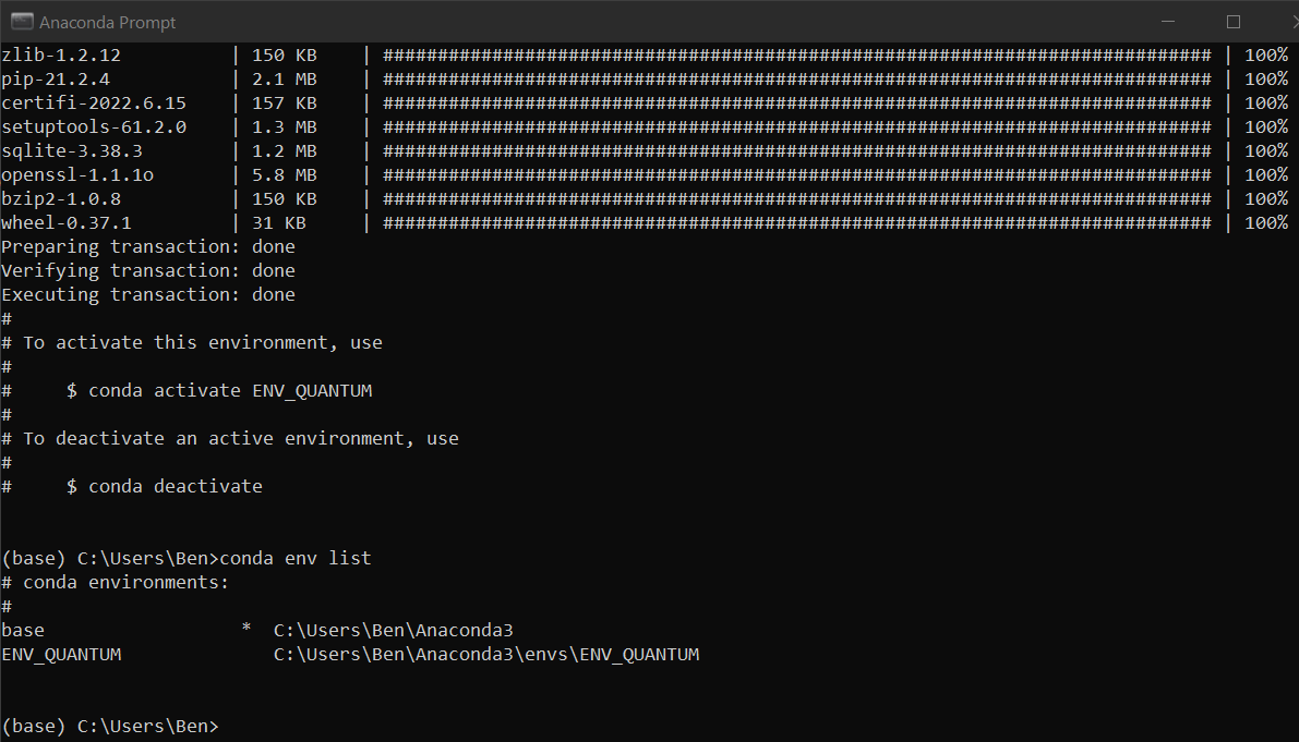
To activate the new environment, type conda activate ENV_QUANTUM. To deactivate the environment type conda deactivate (without the environment name!). Go ahead and try this out.
Let us now install Jupyter Notebook in this new environment. Still in the Anaconda command line we execute:
(ENV_QUANTUM) conda install -c conda-forge notebook
(ENV_QUANTUM) conda install -c conda-forge nb_conda_kernels
Finally, let us install all the Jupyter notebook extensions (when installed properly, it will add a new tab to your Jupyter Notebook session called Extensions).
(ENV_QUANTUM) conda install -c conda-forge jupyter_contrib_nbextensions &&
jupyter contrib nbextension install
A good overview over other extensions: https://towardsdatascience.com/jupyter-notebook-extensions-517fa69d2231.
We will also install the python package manager at this point as well:
(ENV_QUANTUM) conda install pipInstall Qiskit
To install Qiskit in to our Anaconda Environment, simply execute the following in the Anaconda Command Line:
(ENV_QUANTUM) pip install qiskitSince we will be running Qiskit in Jupyter Notebook, we demand the additional visualization functionality. So we also install:
(ENV_QUANTUM) pip install qiskit[visualization]The official install instructions can be found here: https://qiskit.org/documentation/getting_started.html?highlight=conda.
We will also install qiskit_textbook for some nice math output:
(ENV_QUANTUM) pip install git+https://github.com/qiskit-community/qiskit-textbook.git#subdirectory=qiskit-textbook-srcNote that this is not a standard Qiskit package and must be installed from a Git repo.
Start Jupyter Notebook
Deactivate your environment first so that you are back in the BASE environment. Now start a new Jupyter notebook by executing
(ENV_QUANTUM) jupyter notebookA new browser window will pop up showing the file structure at the default path. You’ll want a new folder to contain all of your Jupyter Notebook Projects. I created a new folder called JupyterProjects and then opened it.

Inside the projects folder I will create a new folder called Qiskit and opened it too.
Note that if you want your Jupyter Notebooks to look like mine, just take a look at my blog post here.
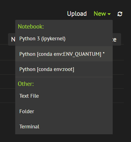
Click the New button drop-down in the top right corner. You should be able to create a new Python File in your own environment:
Hello Quanum World
The first thing we will do is to write a little qiskit program to test out our Jupyter Notebook.
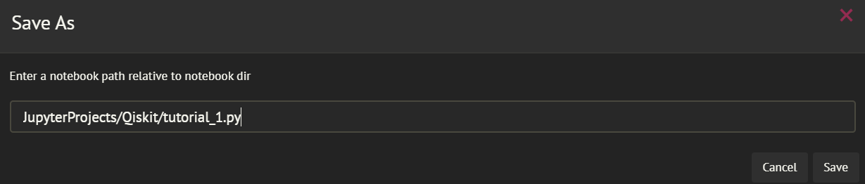
We will follow the same program as per tutorial 1 from the official Qiskit Introduction here. First let us save our notebook as tutorial_1.ipynb:
Typing in the imports:

Then, building a quick quantum circuit (we don’t really need to know what this is just yet!):
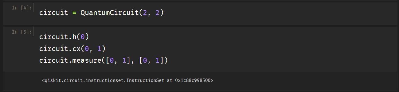
To test the qiskit visualization we can now try to draw this circuit using the draw() method:
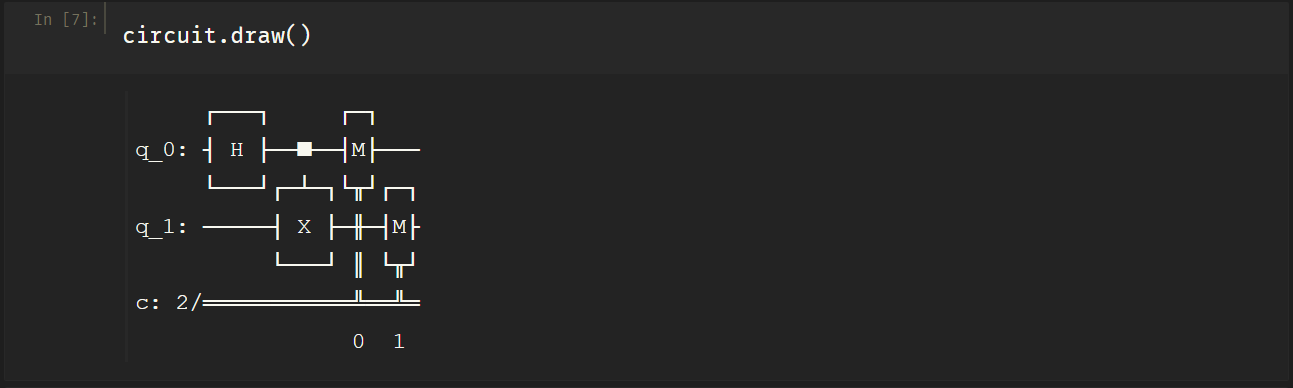
Excellent, as you can see, the circuit visualization worked immediately with my dark Jupyter notebook theme!
Let us now try to visualize the quantum circuit with matplotlib. Inside the draw() parentheses, put the output='mpl' argument like so:
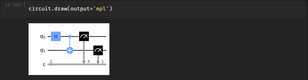
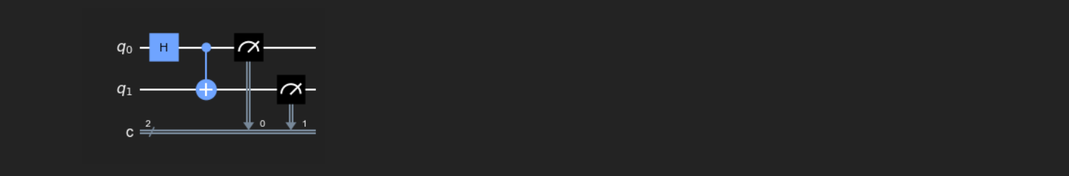
OK, so Qiskit is not going to play nice with my custom Notebook theme. Luckily, we have this resource from Medium, courtesy of Abby Mitchell. So let’s match the theme colours!

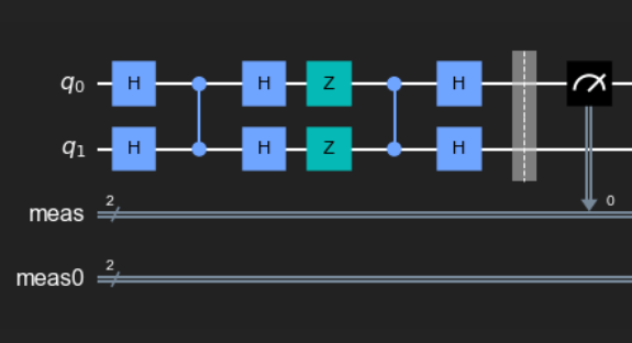
And now the quantum circuit renders nicely with my notebook theme:
2-qubit Grover Circuit
Again, we don’t need to know what or how this circuit operates, but I want to use it as an example to further test our Jupyter Notebook.
The official Qiskit instructions for this particular circuit can be found here.
We start, as usual, with the imports:

In the next cell, we will carry across our custom Qiskit visualisation style:

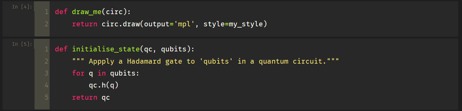
Now some custom functions to help generate the Grover circuit:
Initialising the Grover algorithm looks good:

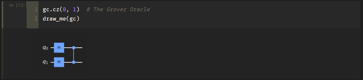
Placing the Grover Oracle:
Finally, the remainder of the circuit:
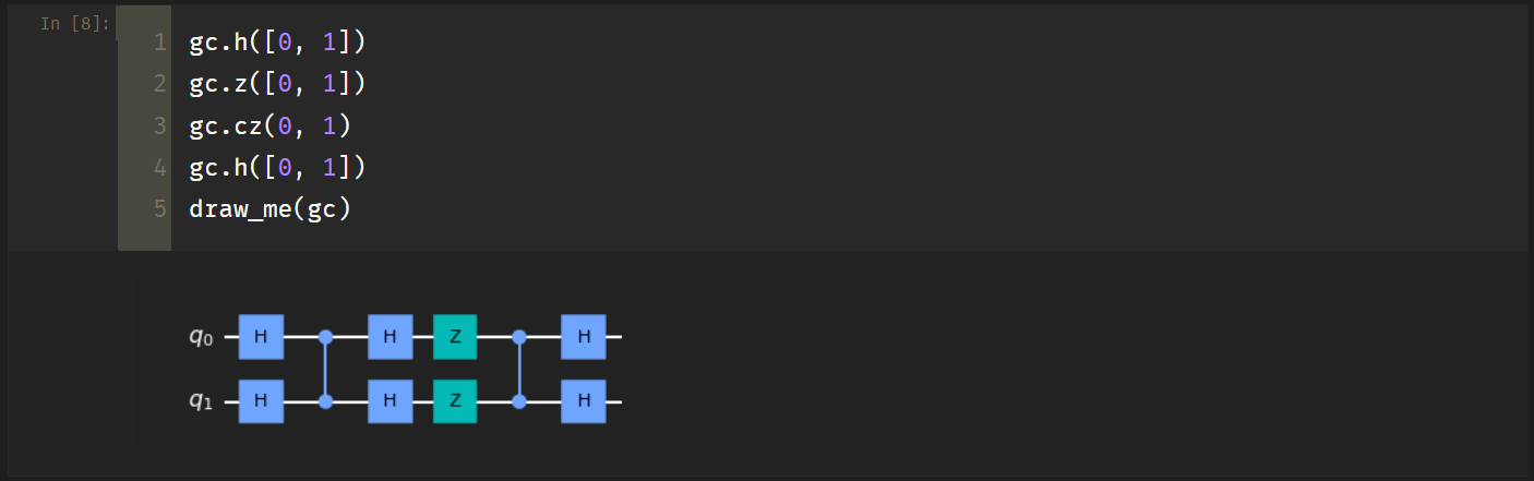
Remember, all of this is just copy-paste from Qiskit.
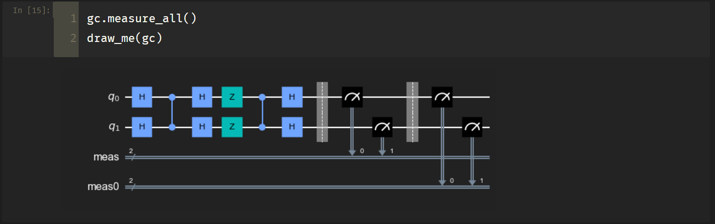
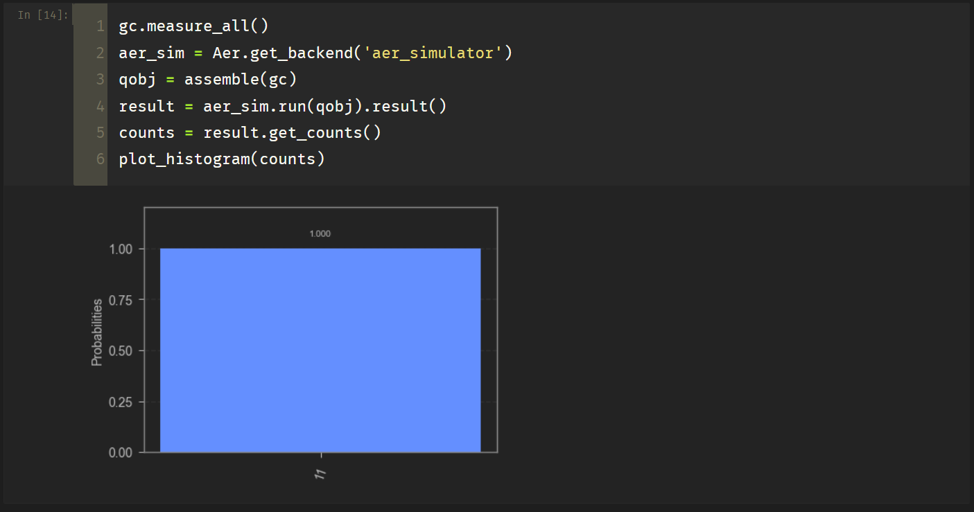
Finally let’s measure the circuit:
Next we will attempt to connect to a quantum simulator:

Histogram Results
Let’s check if the Histogram results work in dark mode:
LaTeX Results
OK, now for the next real test.
We are going to use qiskit_textbook library to see if we can return fancy results!

This is looking good! Note only
As expected, the amplitude of every state that is not 
0, this means we have a 100% chance of measuring 
Amazon Bra-Ket
In the next blog we will extend our setup and config to Amazon Bra-Ket Provider.
References
[1] https://qiskit.org/documentation/intro_tutorial1.html
[3] https://qiskit.org/textbook/ch-algorithms/grover.html#3qubits-simulation
