
Introduction
In the previous article we set up a really simple binomial tree model in Excel and observed that we could artificially change how the random trajectories drifted by altering the probability of moving up and down 


For convenience, here’s what happened.
With the original probability measure, assigning the values of 

Then, we changed probability measure to 
Then we conjectured that the inverse of this exercise must also be true: for a naturally (upward) drifting process, we can cancel-out the drift by changing the probability measure!
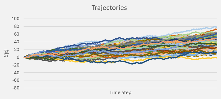
We accomplished this by going to the cells in our worksheet which held the Wiener increments and added in some additive noise. This resulted in a stochastic process (the coin flip stochastic process) with drift 

Then, we played around with the probability measure until it looked like all the drift was gone…

To help find the driftless probability measure, we used a histogram until fitting was good:
Now we shall show an easier, more systematic way of doing this.
Girsanov’s Theorem
The Cameron-Martin-Girsanov theorem (1960), a.k.a. Girsanov’s theorem, is a some-what technical theorem that is used a lot in risk-neutral derivatives pricing. If you want to, click the link above to go to wikipedia and read about it, but for us, here, we don’t need the technical result. Plus, we have already seen Girsanov’s theorem in action! All we need to know is: Girsanov’s theorem tells us that a probability measure (which cancels out drift) simply exists.
But why? Why do we care about driftless stochastic processes?
Cancelling out the drift is actually extremely useful. In fear of swapping one useless term for another: driftless processes are martingales (well, technically local martingales! But that’s too high-brow for us right now). In this blog we will use both “driftless (stochastic) process” and “martingale” interchangebly.
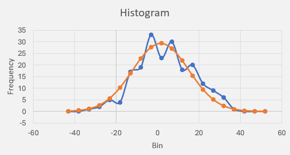
We have already seen what a driftless process looks like. Above, in Fig 1 – the equal-probability coin flip experiment is a martingale.
These martingales are really useful because they have a great property: their next (conditional) expected value is equal to the current value – conditioned on all information up until now. In symbols, this means:
![\displaystyle\mathbb{E}_t^{\mathbb{P}}\left[X_{t+1}|X_{1},\dots,X_{t}\right]](https://s0.wp.com/latex.php?latex=%5Cdisplaystyle%5Cmathbb%7BE%7D_t%5E%7B%5Cmathbb%7BP%7D%7D%5Cleft%5BX_%7Bt%2B1%7D%7CX_%7B1%7D%2C%5Cdots%2CX_%7Bt%7D%5Cright%5D&bg=%23ffffff&fg=%23111111&s=0&c=20201002)
But of course this is true, just look at a driftless process. The mean value of the histogram is always centered at the current value!
It’s constantly resetting itself. In fact, that histogram is really important, because at any point in time, the mean value of the histogram of a driftless process sits in the same spot.
And now we have it!
If the mean value of the empirical histogram of a driftless stochastic process does not change with time, and if that histogram looks like a Gaussian (which is does thanks to the Central Limit Theorem), then for all time, the expectation can be interchanged with a cumulative normal distribution function!
In other words:
![\displaystyle\underbrace{\mathbb{E}_t^{\mathbb{P}}[x_{t+1}|\mathbf{x}_t]}_{\textup{Difficult}} \longrightarrow \underbrace{\Phi(x_t)}_{\textup{Easy}}](https://s0.wp.com/latex.php?latex=%5Cdisplaystyle%5Cunderbrace%7B%5Cmathbb%7BE%7D_t%5E%7B%5Cmathbb%7BP%7D%7D%5Bx_%7Bt%2B1%7D%7C%5Cmathbf%7Bx%7D_t%5D%7D_%7B%5Ctextup%7BDifficult%7D%7D+%5Clongrightarrow+%5Cunderbrace%7B%5CPhi%28x_t%29%7D_%7B%5Ctextup%7BEasy%7D%7D&bg=%23ffffff&fg=%23111111&s=0&c=20201002)
where 
So, basically, expectations become cumulative normals for martingales!
Application
Now for an application.
Let us assume that interest rates are deterministic and that a bank account 


Integrating both sides with respect to time
The 
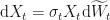
Now we assume that some risky (i.e. stochastic) process 
with constant 


We can dispense with all of the above nonsense and just say that we are operating under the Black-Scholes model, but crucially, this is also all the assumptions we require to quote Girsanov’s theorem (without actually really using it!).
Now introduce a financial instrument, the European call option that pays the following amout at some future time 

where 


We wish to calculate the present value of this instrument at time 

Well, it is common knowledge that the present value will be equal to the expected value of all the discounted future cashflows (conditioned on the sigma-algebra of information received up until pricing time 
![\displaystyle V(0) = \mathbb{E}_0^{\mathbb{P}}\left[V(T)|\mathfrak{F}_0\right]](https://s0.wp.com/latex.php?latex=%5Cdisplaystyle+V%280%29+%3D+%5Cmathbb%7BE%7D_0%5E%7B%5Cmathbb%7BP%7D%7D%5Cleft%5BV%28T%29%7C%5Cmathfrak%7BF%7D_0%5Cright%5D&bg=%23ffffff&fg=%23111111&s=0&c=20201002)
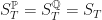
But the future cashflow
![\displaystyle\mathbb{E}_t^{\mathbb{P}}[x_{t+1}|\mathbf{x}_t] \longrightarrow \Phi(x_t)](https://s0.wp.com/latex.php?latex=%5Cdisplaystyle%5Cmathbb%7BE%7D_t%5E%7B%5Cmathbb%7BP%7D%7D%5Bx_%7Bt%2B1%7D%7C%5Cmathbf%7Bx%7D_t%5D+%5Clongrightarrow+%5CPhi%28x_t%29&bg=%23ffffff&fg=%23111111&s=0&c=20201002)
However, the universal pricing theorem says that for any numeraire 
![\displaystyle V(0) = N(0)\times\mathbb{E}_0^{\mathbb{Q}^N}\left[\frac{V(T)}{N(T)}\bigg|\mathfrak{F}_0\right]](https://s0.wp.com/latex.php?latex=%5Cdisplaystyle+V%280%29+%3D+N%280%29%5Ctimes%5Cmathbb%7BE%7D_0%5E%7B%5Cmathbb%7BQ%7D%5EN%7D%5Cleft%5B%5Cfrac%7BV%28T%29%7D%7BN%28T%29%7D%5Cbigg%7C%5Cmathfrak%7BF%7D_0%5Cright%5D&bg=%23ffffff&fg=%23111111&s=0&c=20201002)
…and now this is a martingale under 
But how does this help us? Because we still have a nasty looking expectation there, perhaps even nastier!
Well, it may look nastier but our theorem comes with a clause that says that the process inside the expectation is now a martingale, in other words, the process defined by

is always a martingale under the
So we can use the theorem to reform our present value equation in to one about martingales, then use the martingale property to write it as:
and then claim that this expectation can be evaluated using the approximation
![\displaystyle\mathbb{E}_t^{\mathbb{Q}^N}[x_{t+1}|\mathbf{x}_t] \longrightarrow \Phi(x_t)](https://s0.wp.com/latex.php?latex=%5Cdisplaystyle%5Cmathbb%7BE%7D_t%5E%7B%5Cmathbb%7BQ%7D%5EN%7D%5Bx_%7Bt%2B1%7D%7C%5Cmathbf%7Bx%7D_t%5D+%5Clongrightarrow+%5CPhi%28x_t%29&bg=%23ffffff&fg=%23111111&s=0&c=20201002)
But wait! How do we know what numeraire to use? Where did
How do you Find the Risk-Neutral Probability Measure?
The above universal pricing theorem gets us half-way there.
It got us from the definition of the present value of a future payoff, to an equation involving an expectation of a martingale, with the caveat that the expectation is taken under some equivalent, yet mysteriously unknown probability measure
But it doesn’t tell you how to find the measure! It just says it exists.
So how do we find it?
The short answer is that we don’t need to!
Girsanov’s theorem tells us that a change of measure is synonymous with a change of drift! Right?
Specifically, Girsanov’s theorem intervenes right at the moment when we think all is lost and we need to go and find some mysterious probability measure 
Girsanov Theorem implies that a change of measure is a change of drift!
Okay, but then aren’t we exchanging the problem of: trying to find the right probability measure, with: trying to find the right stochastic differential equation (SDE) with the right drift term
Yes. But the latter problem is easier.
To recap: we don’t brute-force find the 
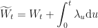
Then, this “right” drift term is obviously the zero drift because we want martingales. So we simply constrain the drift term to zero algebraically, and shunt any compensation to the Wiener process 
…where 
Our SDE, now running with these shunted Wiener increments, 

In other words: instead of trying to find the right measure, we just find under which (algebraic) conditions could we get the SDE to have zero drift, by playing around with the Wiener increments.
If anything this blog is trying to get you to see is: there is more than one way to visualise a change of measure. You can change the probabilities directly: 


Choosing a Numeraire for an Option Payoff
Right. Now that we know what to do, let’s do it.
First, choose a numeraire
Suppose we also have a stochastic asset price 

Now, “Choosing a numeraire” 
where
Now look at that SDE.
Ito promises us that the left-hand side is a martingale under 
Which means we have an available degree of freedom to set this to zero, i.e.

In fact, it is the left-hand side (being promised to be a martingale) that implies that the drift on the right-hand side must be zero, i.e.

So the drift under the new measure is just the risk-free interest rate!
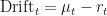
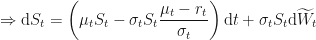
With this intuition in mind, let’s go back to the original SDE and, for ease of notation, let us now define

which gives the SDE as

Let us now factor our 
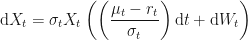
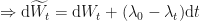
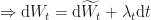
As said before, we now algebraically force this SDE to have zero drift but shunting the excess to the Wiener process. In other words, we substitute
giving
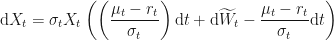
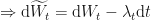
which cancels the drift, and we are left with
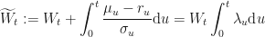
We now invoke Girsanov’s theorem by stating that there must exist an equivalent (martingale) measure 

So, now we have a driftless stochastic process 

To get back to equations in
and substitute it into our original


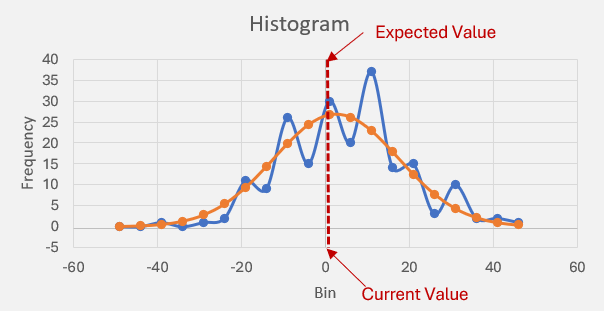
Plotting this SDE will look like this:

with zero drift.
We have not changed anything about the underlying asset 

However, despite these changes, we still have a single, unifying terminal condition: that is:
Conclusion
Now that we have an SDE for the underlying asset under a probability measure that renders it a martingale, allows us to compute expectations (and hence fair value) in a really easy way.
References
- https://en.wikipedia.org/wiki/Girsanov_theorem (1960).
- Igor Girsanov (1934 – 1967).
- Robert H. Cameron (1908 – 1989)
- William T. Martin (1911 – 2004)
