
We are going to try to take a few blog posts and get in to the quantitative mathematics behind the foreign exchange (FX) swap market.
But, as usual in quantitative finance, before we can even get off the ground we need to make a bunch of assumptions.
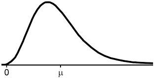
The first assumption is about the FX rate itself. Since FX rates can’t be negative, but at the same time some aspect of them should be Gaussian (normally distributed), we assume that FX rates are distributed Lognormally.
Next, as in (Heath 1992), we assume that the domestic and foreign FX rates are distributed Normally.
Thirdly, we assume that the FX Rate follows a geometric Brownian motion (gBm) over time, with constant drift 

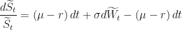
All this means we can write down the equation of evolution of the FX rate as

The Wiener process 
Integrating gives,
![\displaystyle S_t = S_0 \exp\left[\left( \mu - \frac{1}{2}\sigma^2 \right)t + \sigma W_t^{(1)} \right]](https://s0.wp.com/latex.php?latex=%5Cdisplaystyle+S_t+%3D+S_0+%5Cexp%5Cleft%5B%5Cleft%28+%5Cmu+-+%5Cfrac%7B1%7D%7B2%7D%5Csigma%5E2+%5Cright%29t+%2B+%5Csigma+W_t%5E%7B%281%29%7D+%5Cright%5D+&bg=%23ffffff&fg=%23111111&s=0&c=20201002)
…and this is about as far as we can go without introducing more assumptions.
First of all, it should be noted that as it is written, the FX Rate price 
Unfortunately however, the FX Rate, as it is written, is not yet a martingale…and it won’t be, unless 
In what follows we will discuss how to obtain the right martingale, and why this quest is a worthwhile one.
The Quest for the Holy Martingale
We seek a martingale.
Martingales are, by definition, driftless.
So, is there is some logical way to transform the drift out of the equation? In a similar fashion to Lebesgue integration (see my article here), we can change the probability measure so that the drift term vanishes all by itself, and we don’t have to set it equal to zero.
We are going to change the probability measure so that the drift term vanishes all by itself!
In other words, we want a naturally driftless process looking like this:

The tildes are there to indicate that we want the symbols of our equations to be related but they are slightly different to the original values. Namely, the probability measure 
Changing the Measure
Here is an example of how we can change the probability of measure of a simple stochastic system: the 6-sided die.
A 6-sided die has 6 possible outcomes, 6 faces which could show up. These faces are labels and we list them out here. Faces and Labels have no mathematical substance, so we must map a face to a number. In this case it is obvious which map to use because the face/label indicates precisely which integer to use, i.e. 1 dot maps to the number 1, 2 dots map to 2, and so on. This is what a random variable does: it maps faces/labels/events to numbers.
Now that we have numbers to play with we utilise the probability measure to further map the integer to a probability. Thus, in our simple model, we have done the following mapping:
![\displaystyle\mathcal{F} \ni \sigma \mapsto \mathbb{Z} \mapsto [0,1] \subseteq \mathbb{R}](https://s0.wp.com/latex.php?latex=%5Cdisplaystyle%5Cmathcal%7BF%7D+%5Cni+%5Csigma+%5Cmapsto+%5Cmathbb%7BZ%7D+%5Cmapsto+%5B0%2C1%5D+%5Csubseteq+%5Cmathbb%7BR%7D&bg=%23ffffff&fg=%23111111&s=0&c=20201002)
We have to do this everytime we employ a probability model.
OK, now we can draw some things. In what follows we have a so-called fair die which has a equal probability of turning up any of the six faces. Since probabilities must sum to 100%, each face is assigned a probability of 16.67%.
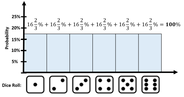
This probability distribution is a result of the following probability measure:
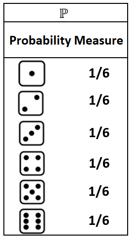
Now, let us see what happens when we change the measure:
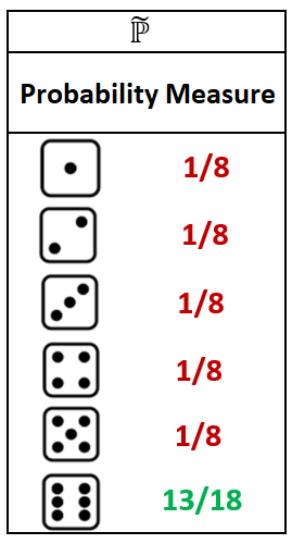
This is a rigged or unfair die as this die rolls a 6 much more often than any other result. And now, the experiment looks different:
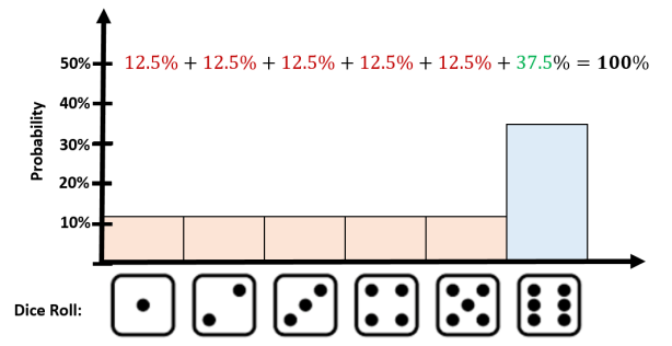
The point I want to make is that in probability theory we are free to change our probability measure whenever our experiments are not working. In this example we were trying to model an unfair die and clearly the first probability measure was not matching what we were observing in reality. Exchanging that measure for the second one allowed us to match reality much more accurately.
We do the same thing in quantitative finance. The probability measure that comes with the BSM model is the so-called real world probability meaure 
But you see, we do not state such changes in probability measure without also stating what our reason for changing is. In the die example, we had an unfair die, so the re-weighting of the measure was due to that. For the risk-neutral measure
We do not have to use the Money Market account either. We can have experiments in quantitative finance where some other interaction with some other financial asset dictates a change in measure. But only some assets work and make sense for this. We call these assets numéraires, and they are very useful for changing the probability measure to suit experimental evidence. But more on that later.
Why Do We Want Martingales?
Martingales are useful.
An important feature of martingales is Doob’s Optional Stopping Theorem which says that the expectation of a martingale is constant in time, even if we randomly stop it.
An important example of a martingale is Brownian motion (geometric Brownian motion is not!).
Martingales have their own convergence theorems, which are really only useful in proving subtle, technical details outside the scope of this article.
Another nice technical feature of Martingales are that they are decomposable.
Technical qualities aside, they are also highly practical. Indeed, in quantitative finance, martingales are absolutely crucial for pricing. Here’s why.
Crucial for Pricing
The Fundamental Theorem of Asset Pricing (FTAP)is a mathematical theorem that provides the necessary and sufficient conditions for a financial market (an environment where things are traded at varying prices between a large number of people) to be arbitrage-free and complete (which is a fancy way of saying: “Hey! No risk-less profit, no transactional costs, perfect information, and there is a price for everything!”).
While this sounds like a lot of fluff, all these economic statements can and have been boiled down to a simple statement about the existence of a sacred, mysterious probability measure, called the risk-neutral measure, often denoted by
Could this be what we will transform
A corollary of the Fundamental Theorem of Asset Pricing then says that if one happens to have a complete, arbitrage-free market, then any derivative’s price is equal to the discounted expected value of future cashflows (payoffs) under the risk-neutral measure. The existence of this risk-neutral measure is therefore a direct result of the no-arbitrage claim.
Another name of the risk-neutral measure
If we believe in the FTAP then we believe that there is only ever one, unique EMM. This implies that there is only ever one, unique price for each asset in the market. And this is a very important belief, because we surely can’t have two different prices for the same thing!
We need the FTAP to believe that there is a unique price for each asset. But to realise the unique price, we need to re-weight all of our real-world probabilities in to risk-neutral ones. Then (and only then) do our asset prices start behaving like driftless martingales.
If there is no EMM then this is equivalent to the existence of arbitrage opportunities.
And, as you can see, the solution was not as simple as setting
So How Do We Get a Martingale?
OK, so Martingales sound pretty awesome, and they are! But how do we get one?
Well, we’ve hinted that it has something to do with changing the probability measure. This change has the power to make the drift in the FX Rate stochastic process vanish. But, unfortunately, this change also affects the very properties of the Wiener process driving the thing. So we must proceed with caution!
The challenge is to not only find a new, equivalent probability measure but also a new random Wiener process to go with it. This new random process need to be suitably random under the EMM as well, we can’t just use the old one.
So we need to transform 

Ugh! Sounds tough.
Well, whatever the new random process
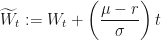
If we substitute this in, we get
![\displaystyle S_t = S_0 \exp\left[\left( \mu - \frac{1}{2}\sigma^2 \right)t + \sigma\left( \widetilde{W}_t - \left( \frac{\mu - r}{\sigma} \right)t \right) \right]](https://s0.wp.com/latex.php?latex=%5Cdisplaystyle+S_t+%3D+S_0+%5Cexp%5Cleft%5B%5Cleft%28+%5Cmu+-+%5Cfrac%7B1%7D%7B2%7D%5Csigma%5E2+%5Cright%29t+%2B+%5Csigma%5Cleft%28+%5Cwidetilde%7BW%7D_t+-+%5Cleft%28+%5Cfrac%7B%5Cmu+-+r%7D%7B%5Csigma%7D+%5Cright%29t+%5Cright%29+%5Cright%5D+&bg=%23ffffff&fg=%23111111&s=0&c=20201002)
![\displaystyle \text{...} = S_0 \exp\left[\left( \mu - \frac{1}{2}\sigma^2 \right)t + \sigma \widetilde{W}_t - \left( \frac{\mu - r}{\sigma} \right)\sigma t \right]](https://s0.wp.com/latex.php?latex=%5Cdisplaystyle%C2%A0+%5Ctext%7B...%7D+%3D+S_0+%5Cexp%5Cleft%5B%5Cleft%28+%5Cmu+-+%5Cfrac%7B1%7D%7B2%7D%5Csigma%5E2+%5Cright%29t+%2B+%5Csigma+%5Cwidetilde%7BW%7D_t+-+%5Cleft%28+%5Cfrac%7B%5Cmu+-+r%7D%7B%5Csigma%7D+%5Cright%29%5Csigma+t+%5Cright%5D+&bg=%23ffffff&fg=%23111111&s=0&c=20201002)
![\displaystyle \text{...} = S_0 \exp\left[\left( \mu - \frac{1}{2}\sigma^2 \right)t + \sigma \widetilde{W}_t - \left( \mu - r \right) t \right]](https://s0.wp.com/latex.php?latex=%5Cdisplaystyle%C2%A0+%5Ctext%7B...%7D+%3D+S_0+%5Cexp%5Cleft%5B%5Cleft%28+%5Cmu+-+%5Cfrac%7B1%7D%7B2%7D%5Csigma%5E2+%5Cright%29t+%2B+%5Csigma+%5Cwidetilde%7BW%7D_t+-+%5Cleft%28+%5Cmu+-+r+%5Cright%29+t+%5Cright%5D+&bg=%23ffffff&fg=%23111111&s=0&c=20201002)
![\displaystyle \text{...} = S_0 \exp\left[\left( r - \frac{1}{2}\sigma^2 \right)t + \sigma \widetilde{W}_t \right]](https://s0.wp.com/latex.php?latex=%5Cdisplaystyle%C2%A0+%5Ctext%7B...%7D+%3D+S_0+%5Cexp%5Cleft%5B%5Cleft%28+r+-+%5Cfrac%7B1%7D%7B2%7D%5Csigma%5E2+%5Cright%29t+%2B+%5Csigma+%5Cwidetilde%7BW%7D_t+%5Cright%5D+&bg=%23ffffff&fg=%23111111&s=0&c=20201002)
…and, darn! We still have a drift term. Further, we have only succeeded in replacing the 
Let’s try something else.
Let us try to transform the FX Rate 
In other words, let’s define 

Then we get:
![\displaystyle e^{rt}\widetilde{S}_t = S_0 \exp\left[\left( \mu - \frac{1}{2}\sigma^2 \right)t + \sigma\left( \widetilde{W}_t - \left( \frac{\mu - r}{\sigma} \right)t \right) \right]](https://s0.wp.com/latex.php?latex=%5Cdisplaystyle+e%5E%7Brt%7D%5Cwidetilde%7BS%7D_t+%3D+S_0+%5Cexp%5Cleft%5B%5Cleft%28+%5Cmu+-+%5Cfrac%7B1%7D%7B2%7D%5Csigma%5E2+%5Cright%29t+%2B+%5Csigma%5Cleft%28+%5Cwidetilde%7BW%7D_t+-+%5Cleft%28+%5Cfrac%7B%5Cmu+-+r%7D%7B%5Csigma%7D+%5Cright%29t+%5Cright%29+%5Cright%5D+&bg=%23ffffff&fg=%23111111&s=0&c=20201002)
![\displaystyle \widetilde{S}_t = S_0 \exp\left[\left( \mu - r - \frac{1}{2}\sigma^2 \right)t + \sigma\left( \widetilde{W}_t - \left( \frac{\mu - r}{\sigma} \right)t \right) \right]](https://s0.wp.com/latex.php?latex=%5Cdisplaystyle+%5Cwidetilde%7BS%7D_t+%3D+S_0+%5Cexp%5Cleft%5B%5Cleft%28+%5Cmu+-+r+-+%5Cfrac%7B1%7D%7B2%7D%5Csigma%5E2+%5Cright%29t+%2B+%5Csigma%5Cleft%28+%5Cwidetilde%7BW%7D_t+-+%5Cleft%28+%5Cfrac%7B%5Cmu+-+r%7D%7B%5Csigma%7D+%5Cright%29t+%5Cright%29+%5Cright%5D+&bg=%23ffffff&fg=%23111111&s=0&c=20201002)
But now we need to get back to the representation of this as 
Define 


and so we have:


Ito’s Lemma:


Substituting in our known expression for 


…and we get:

Oh no! There is still that pesky drift term in there!
So, two attempts at naïve transformation has not achieved the aim that is to remove the drift term.
However, it is clear from the last line above that the process 

So what if we try the above transformations together?
Starting with our last expression:


Awesome! No drift term.
Our wild guess at
worked perfectly for the process
Why?
The reason it worked for the tilde process
Recall that to get
Well, it just so happens that 

But why did this work? What is so special about normalising asset prices with a zero-coupon bond?
Numéraire
What we did above was not only wild guessing, but was essentially a transformation of the FX Rate prices in to a new FX Rate price without introducing any new form of risk (i.e. randomness).
If your price process is completely deterministic (no randomness) then it can always be used as a numéraire, i.e. it can be used to normalise the main, risky price process.
Examples of numéraires are:
- Money Market Account,
- Currency Exchange Rates,
- The Forward Numeraire (zero-coupon bond),
- Annuities
The numéraire itself can be discounted

and will also be a martingale under the transformed probability measure 
Guessing for Days…
There is a better way of finding the transformation
that works rather than wild guessing?
Yes. It’s called Girsanov’s Theorem and we will cover it in the next blog post and show why how we finally get and use a martingale, why numéraire’s work for us, and then explain what we set out to do: pricing in the foreign exchange swap market.
But for now, let me wrap up with a quick summary of what we really do in practice (instead of guessing):
- Pick a suitable numéraire
,
- Make sure that the ratio
takes a sufficiently simple form,
- use Girsanov’s Theorem to determine the dynamics of
and we will see exactly how to perform Step 3 in the next blog.
