
Introduction
In this blog we are going to extend our knowledge of Markov chains that was discussed in the previous blog post here. We will be again working in a probability space, and note that there is a correspondence between Markov chains, graphs, and transition matrices which is illustrated by the top of the mind map here:

As you can see, there is a bit to cover in this blog! We have already seen how we can encode our Markov chain in to a transition matrix:the square matrix whose rows sum to 1 and contains all the individual probabilities for transitioning from state to state. We also formed the eigenvalue-eigenvector (EE) problem in the last blog to motivate the definition of a Markov chain stationary distribution – basically, the histogram of all its states by how many times that state is visited if one is left to traverse the chain in an infinite amount of time.
In this article, however, the EE problem will form the basis of defining the spectrum of a Markov chain and, in turn, its spectral radius. Both of these properties are crucial ingredients in the Gershgorin circle theorem which provides the result that the spectral radius of the Markov chains that we will be dealing with all have value 1. This particular value, along with Brouwer’s fixed point theorem ensures that this property always exists for all the Markov chains we’ll be interested in.
Finally, we employ the Perron-Frobenius theorem to define yet another Markov chain property known as its spectral gap, which is an important input in to a measuring device known as the total variational distance which is used to describe the Markov chain’s Mixing Time, our aim for this blog post.
Note that we also had to add a little bit of structure to our probability space, namely, we had to add a metric to it. This is fine, not too much to worry about. But, without it, we wouldn’t have been able to define the total variational distance.
So let’s get cracking!
Motivation
We are going to need a bit of motivation for bothering to define a Markov chain’s mixing time.
Our primary motivation comes in the form of Bayes’ theorem.

How does this work?
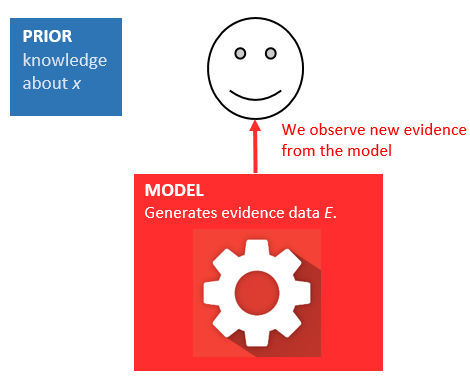
OK, so we start with some prior, usually pretty inaccurate knowledge about some parameter 

…and we usually have some model that produces data that we call Evidence:

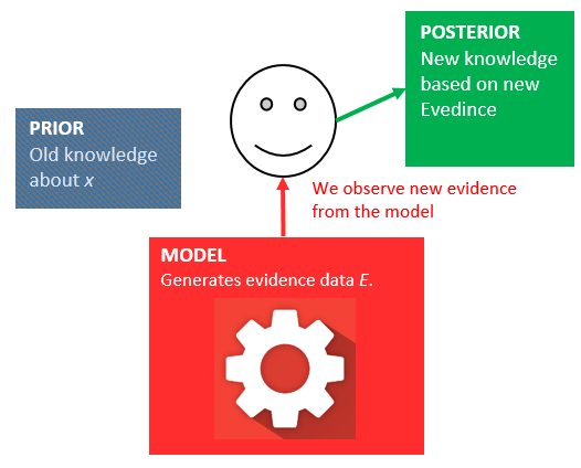
We observe new evidence from the model:
…and update our belief about our prior knowledge:
But we can’t always assume that the model produces accurate evidence! Maybe one time it provides some outlier evidence, or even just wrong evidence. To compensate for this, and to make sure we aren’t just completely discarding our prior knowledge, we mix the new evidence with a likelihood rating that’s dependent on our prior knowledge; almost like a security guard or firewall that protects our belief against bad data:
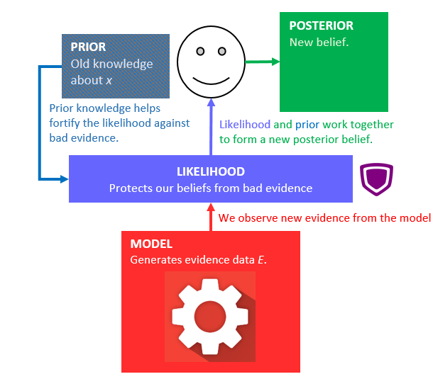
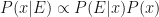
Thus, Bayes’ theorem says that the posterior probability is proportional to the product of the prior probability and the likelihood function (the security guard).
Proportional can be interpreted as having to divide by some “constant” to ensure that a probability of 1 is assigned to the whole space, this is an axiom of probability theory, so we can’t violate it! But this divisor (the evidence) is the nasty piece of the puzzle.
To get to this “constant“, consider a hypothesis (basically just a vector of data points) 


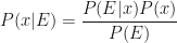
All four quantities are combined in to a Bayes’ theorem:
If we try to be a little more general, then we can remove the divisor from the above formula and replace the equals sign with a proportional sign:
Monte Carlo Markov Chains
So, we choose to believe and follow Bayes’ theorem. Here it is again for convenience:
and we want to calculate the posterior probability distribution 
Since this normalising constant is what makes Bayes’ theorem so difficult to implement in a computer we have to approximate the posterior
So, two things going on here: 1) we’ve jumped from Bayes’ theorem to something called a Markov chain, and 2) what on Earth is a Monte Carlo method?
Well, Monte Carlo methods are a broad class of algorithms that rely on repeated sampling to obtain numerical results. We are not going to talk about how Monte Carlo algorithms work in this blog, but instead we will note that there are two, very powerful engines running beneath the covers: the Central Limit Theorem (CLT), which turns independent random variables in to normally distributed random variables:

Therefore, if we draw enough samples according to the Law of Large Numbers, from any probability distribution, then the Central Limit Theorem says that even if we don’t know what it should be then we can compute a Monte Carlo estimate to arrive at a good approximation of some expectation.
The key takeaway: we don’t need to even have the full probability distribution for this to work. We just need enough samples!
OK, cool. So we’ll just make up some distribution and start drawing samples?
After that, one progresses to importance sampling (IS) which pretty much works for everything. But there are some, very important, integrals that even IS doesn’t do well.
Here is a interesting illustration to show how a Markov chain can generate a probability distribution

The Idea Behind MCMC
OK, so we need to approximate the posterior distribution by approximating the denominator of Bayes’ formula. We are going to do this by drawing samples from a probability distribution. Which probability distribution? The stationary distribution of a Markov chain! (we didn’t spend a whole blog post talking about that for nothing!) So we create a Markov chain whose stationary distribution is the one we want to sample from, then we just simulate a sequence of states and generate a histogram of the frequency each state is reached by pretending to transition around the chain:

This acts as the probability distribution we want to sample from. There is no function to tell you what the height of each bar is. Yet there is a clear link between the height of this distribution and the amount of time spent at each state in the Markov chain. We don’t use all the state values, that wouldn’t be wise at all. Instead we just keep some of the state values, particularly those well into the run – as far from the beginning as possible.
We need to wait for the Markov chain pie to reach its steady state temperature before it is ready to eat!
We can’t even keep successive samples from the Markov chain because by its very definition there is a strong correlation between any two neighbouring states. It’s a bit involved, but basically we have to look at the autocorrelation plots of the sequence to ensure independence of samples. But that’s not too hard to do. Once we have the empirical distribution created from the Markov chain. We can then sample it using acceptance-rejection much like the following illustration describes:

Here is a interesting illustration to show how a Markov chain can generate a probability distribution:
Conclusion
Markov Chain Monte Carlo (MCMC) algorithms are perhaps the most popular sampling method for Bayesian Inference as they provide flexible and powerful solutions to approximate the posterior distribution, and they are easy to implement regardless of dimension and non-linearity. However, the performance of MCMC algorithms strongly depend on its initial tuning and acceptance-rejection rules. We didn’t talk much about the tuning aspect of the Markov chain and I will leave that to the next article on this subject. But I would like to state that the convergence of the Markov chain to the stationary distribution is a long and arduous process. The convergence is generally poor. In the next article I
Explanation of MCMC by Rich
I really like this explanation of a Markov Chain Monte Carlo, see ref [1]:
Anytime we want to talk about probabilities, we’re really integrating a density. In Bayesian analysis, a lot of the densities we come up with aren’t analytically tractable: you can only integrate them — if you can integrate them at all — with a great deal of suffering. So what we do instead is simulate the random variable a lot, and then figure out probabilities from our simulated random numbers. If we want to know the probability that X is less than 10, we count the proportion of simulated random variable results less than 10 and use that as our estimate. That’s the “Monte Carlo” part, it’s an estimate of probability based off of random numbers. With enough simulated random numbers, the estimate is very good, but it’s still inherently random.
So why “Markov Chain”?
Because under certain technical conditions, you can generate a memoryless process (aka a Markovian one) that has the same limiting distribution as the random variable that you’re trying to simulate. You can iterate any of a number of different kinds of simulation processes that generate correlated random numbers (based only on the current value of those numbers), and you’re guaranteed that once you pool enough of the results, you will end up with a pile of numbers that looks “as if” you had somehow managed to take independent samples from the complicated distribution you wanted to know about.
“So for example, if I want to estimate the probability that a standard normal random variable was less than 0.5, I could generate ten thousand independent realizations from a standard normal distribution and count up the number less than 0.5; say I got 6905 that were less than 0.5 out of 10000 total samples; my estimate for P(Z<0.5) would be 0.6905, which isn’t that far off from the actual value. That’d be a Monte Carlo estimate. “Now imagine I couldn’t draw independent normal random variables, instead I’d start at 0, and then with every step add some uniform random number between -0.5 and 0.5 to my current value, and then decide based on a particular test whether I liked that new value or not; if I liked it, I’d use the new value as my current one, and if not, I’d reject it and stick with my old value. Because I only look at the new and current values, this is a Markov chain. If I set up the test to decide whether or not I keep the new value correctly (it’d be a random walk Metropolis-Hastings, and the details get a bit complex), then even though I never generate a single normal random variable, if I do this procedure for long enough, the list of numbers I get from the procedure will be distributed like a large number of draws from something that generates normal random variables. This would give me a Markov Chain Monte Carlo simulation for a standard normal random variable. If I used this to estimate probabilities, that would be a MCMC estimate.
References
[1] https://stats.stackexchange.com/questions/165/how-would-you-explain-markov-chain-monte-carlo-mcmc-to-a-layperson [2] https://www.researchgate.net/publication/334001505_Adaptive_Markov_chain_Monte_Carlo_algorithms_for_Bayesian_inference_recent_advances_and_comparative_study
However, if the Markov Chain is finite (but usually very long), aperiodic, irreducible, and ergodic (just as we talked about before) then, quite amazingly, the samples will be drawn from the desired posterior distribution!
However, if the Markov Chain is finite (but usually very long), aperiodic, irreducible, and ergodic (just as we talked about before) then, quite amazingly, the samples will be drawn from the desired posterior distribution!
