
It only took 3 years to upgrade the revolutionary Black-Scholes-Merton (BSM) model of 1973 [2] so that it could handle commodities.
But why did it need upgrading for commodities?
The BSM Model
To answer this, let us first remind ourselves of the main assumptions of the BSM model that revolutionised the pricing of options on equities:
- there exists a risk-free interest rate,
- the underlying asset (e.g. an equity) follows a geometric Brownian motion,
- the underlying asset does not pay a dividend,
- it is possible to borrow and lend any amount of money (even fractional) at the risk-free rate,
- it is possible to buy or sell any amount of the underlying (even fractional),
- there are no arbitrage opportunities,
- all the transactions above do not incur any fees or costs (i.e. frictionless market).
Within assumption #2 of geometric Brownian motion lies further assumptions that:
- The drift and volatility are constant and non-random.
And this is where the problems begin…
The Problem With Assuming
You see, by assuming that your underlying asset follows a geometric Brownian motion you are also assuming that the logarithm of the asset value follows a regular Brownian motion with drift.
How do we know that the price of derivatives follows such assumptions?
Well, they don’t – not exactly…
They just sort-of appear like they do, and, of course, every so-often they don’t at all! (c.f. https://en.wikipedia.org/wiki/Financial_crisis for a list of 50 instances where they didn’t!)
So what we can say is that the price of a derivative, call it 
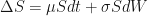
which says that a small change in the price of a derivative is equal to some random process (the 

If you graph this equation for different levels of drift and volatility over time you get something that looks like this:

That graph looks pretty convincing, right? In fact, statistically speaking, you’d have a hard time convincing yourself that it wasn’t realistic; which is why this model has been so good at approximating the real price of a derivative for the past 47 years.
OK, so this assumption allows us to model the evolution of the underlying asset price. What about the price of the derivative?
If we assume that drift and volatility are constant (recall this is the assumption we inherit when we assume a geometric Brownian motion) then the only other variables that could possibly drive the value of a derivative is the underlying asset price 
Thus, we need to know how the value of a derivative 
But our assumptions have forced us to consider another function 
Ito’s Lemma
So how do we get from
to

We won’t get in to the details in this blog but what we do is make another assumption on 


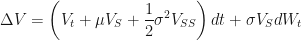
where 


Removing Randomness
This (Ito’s Lemma) equation still has a lot of randomness in it, note that 
A bold endeavour. Let’s see how it is done…
Imagine I give you a portfolio, with value 


Now we discretize time, allowing the value of this portfolio to evolve to the future time 


and the
If the uncertainty has been eliminated then the portfolio must be risk-free.
If the portfolio is risk-free it must generate returns equal to the risk-free interest rate (otherwise arbitrage opportunities would exist).
The risk-free interest rate over the period from 


We know what 

Simplifying by collecting terms and equating one side to be zero we get the celebrated Black-Scholes partial differential equation (PDE):

This PDE can be solved analytically assuming a bunch of boundary conditions:
- When the underlying asset price is 0, the value of the derivative is 0,
- The value of the derivative approaches the value of the underlying asset as the value of the asset approaches infinity (which also happens when the volatility of the underlying asset approaches infinity)
- The value of the derivative equals
, where
is the derivative’s strike price, at maturity when
, i.e. the functional form of the value is known at maturity.
The solution of the Black-Scholes PDE is achieved by noting that it is a Cauchy-Euler equation which can be transformed in to a diffusion equation via the change of some variables. Under these changes the PDE actually reduces to a well-known form:

where 

Due to the change of the elapsed-time variable 

The next steps are quite convoluted (pun intended), and outside the scope of this blog post. For the interested reader, follow pages 33 to 40 of Robert Buchanan’s slides here for more information, or stackexchange here. But in the end we end up with the solution

where 

The form of this solution as essentially 

I might think about creating a separate blog post dedicated to this solution. If I do, I will link it here.
Relaxing Assumptions
Right, well. That was a lot! But now that we have all of the technical stuff out of the way we have earned ourselves a breather, so let us relax some of the many assumptions of Blacks, Scholes and Merton and see what happens…
In 1976, Fischer Black (1938-1995) did just this! You see, there was a disconnect between the value of options on commodities as traders saw them, and as risk management saw them. The idea at the time was that that somehow, the price of the underlying commodity wasn’t playing by all the rules as requested by Black, Scholes and Merton. So Fischer Black found a way around the problem:
He published a paper that modelled the futures prices, instead of the spot prices of commodities, that appeared to be immune to the non-randomness…
For futures under the BSM framework, margin calls essentially kill off any drift, which means we need to model them slightly differently.
Intuitively, futures should have zero drift (a.k.a. they’re driftless) because entering in to a futures contract is always going to cost you nothing up front, and nothing doesn’t drift! Futures contracts are then continuously marked-to-market requiring payments equal to margin calls; and it’s these margin calls that essentially kill off any drift.
One way to view the Black-76 formula is as the Black-Scholes model with a continuous dividend yield equal to the risk-free interest rate.
Take a look at one of the eight assumptions of the BSM model, that is: “the underlying asset is log-normally distributed“. Now consider the spot price (the immediate price) an agricultural product, or an energy product, which is clearly not random. Agriculturals will typically rise prior to harvest season and fall immediately following the harvest. The same with energy products such as natural gas; they’re more expensive in winter and less so in summer (at least in the Northern Hemisphere). Therefore there is an element of predictability for these things.
Predictability violates the Black-Scholes-Merton model!
This non-randomness of spot commodities actually invalidates the use of the Black-Scholes-Merton model because they will refuse to follow Brownian motion, and hence, they violate one of those core assumptions.
So, instead of modelling spot prices, Fischer Black modelled futures prices. In other words: the underlying in Black-76 is a futures price instead of a spot price.
Futures instead of Spot
OK, so what did this do?
Well, first of all, spot equals futures at expiry. So no difference there; at that boundary there is literally no difference between the two.
We can eliminate another degree of freedom by observing that the spot price of a futures contract is always zero. This causes the value of any long position in the futures contract to vanish.
So, in light of this, let’s begin with the futures price 


![\displaystyle F(t;T_d) = \mathbb{E}_t^{\mathbb{Q}}\left[S_T | \mathcal{F}_t\right]](https://s0.wp.com/latex.php?latex=%5Cdisplaystyle+F%28t%3BT_d%29+%3D+%5Cmathbb%7BE%7D_t%5E%7B%5Cmathbb%7BQ%7D%7D%5Cleft%5BS_T+%7C+%5Cmathcal%7BF%7D_t%5Cright%5D&bg=%23ffffff&fg=%23111111&s=0&c=20201002)
where
The Quest for a Suitable Numeraire
Problem Fischer Black faced now is: what is the suitable numeraire?
He found that if there exists a suitable bond in the marketplace with just the right maturity date and interest rate then using it as a numeraire (and Girsanov’s theorem) allows us to write the above equation as
![\displaystyle F(t;T_d) = \mathbb{E}_t^{\mathbb{Q}}\left[S_T | \mathcal{F}_t\right] = B_T \mathbb{E}_t^{\mathbb{Q}}\left[\frac{S_T}{B_T}|\mathcal{F}_t\right]](https://s0.wp.com/latex.php?latex=%5Cdisplaystyle+F%28t%3BT_d%29+%3D+%5Cmathbb%7BE%7D_t%5E%7B%5Cmathbb%7BQ%7D%7D%5Cleft%5BS_T+%7C+%5Cmathcal%7BF%7D_t%5Cright%5D+%3D+B_T+%5Cmathbb%7BE%7D_t%5E%7B%5Cmathbb%7BQ%7D%7D%5Cleft%5B%5Cfrac%7BS_T%7D%7BB_T%7D%7C%5Cmathcal%7BF%7D_t%5Cright%5D&bg=%23ffffff&fg=%23111111&s=0&c=20201002)
Ugh, this looks more complicated.
Well, it isn’t. The fraction 

which says that the price, at time 
What does the long holder of a (European) call option see?
Well, at maturity of the option 

where 
But we know what 
Substituting that in to the formula for the payoff, and we get:

Problem here is that to proceed under the BSM model we need the exercise price to be all by itself in the formula, and we have that pesky factor of 

Now 

But setting 

So, before settlement, then, we go back to basics and look at the basic call 


where the replacement of spot with futures is also replaced in the auxillary parameters:


and, as usual, 

And just from this, we can even calculate fairly typical examples like this one from the London Metal Exchange website: Worked Example from LME.com.
Conclusion
There is nothing stopping us from replacing the underlying asset in the Black-Scholes-Merton (BSM) model with a futures asset. In the words of Fischer Black himself:
…the futures price is the price at which we can agree to buy or sell an asset at a given time in the future without putting up any money now.
References
[1] Black, F. “The pricing of commodity contracts“, Journal of Financial Economics 3, ppg 167-179 (1976)
[2] Black, F. & Scholes, M. “The pricing of Options and Corporate Liabilities“, Journal of Political Economy 81, ppg 637-654 (1973)
[3] Merton, R. C. “Theory of rational option pricing“, The Bell Journal of Economics and Management Science, 4(1), ppg 141-183 (1973)
[4] Margrabe, W. “The value of an option to exchange one asset for another“, Journal of Finance 33(1), ppg 177-186 (1978)
[5] Garman, M. K. & Kohlhagen, S. W. “Foreign currency option values“, Journal of International Money and Finance 2(3), ppg 231-237 (1983)

In the LME example, taking the call price as an example, the discount factor $e^{-r(T+2/52)}$ adjust the time to include the days to futures prompt day, which is different from the $e^{-r(T-t)}$ here considering the days to options expiry? Anything I missed?