I never spent much time thinking about the Quadratic variation of a random process when I was first studying stochastic calculus. It turns out that it sits right at the heart of the definition of the Ito integral, the workhorse of stochastic calculus. A consequence of my ignorance was that when it came time to use a quadratic variation argument (say for instance in the a final exam) I was never able to make my solution very convincing.
So recently I decided I would sit down and try to understand exactly what quadratic variation is, why is was so important and when was the correct time to use it.
In order to talk about the quadratic variation of a random process we need a probability space (a sample space 


![\left[X\right]_t := \lim\limits_{\|P\|\rightarrow 0} \displaystyle\sum_{k=1}^n \left( X_{t_k} - X_{t_{k-1}} \right)^2](https://s0.wp.com/latex.php?latex=%5Cleft%5BX%5Cright%5D_t+%3A%3D+%5Clim%5Climits_%7B%5C%7CP%5C%7C%5Crightarrow+0%7D+%5Cdisplaystyle%5Csum_%7Bk%3D1%7D%5En+%5Cleft%28+X_%7Bt_k%7D+-+X_%7Bt_%7Bk-1%7D%7D+%5Cright%29%5E2++&bg=ffffff&fg=000000&s=0&c=20201002)
There’s quite a bit going on in this defintion. There is a partition of time, a mesh going to zero, and a sum of squared differences. Another interesting remark that is often overlooked is that the quadratic variation is actually itself a stochastic process, it has a value for each point in time (note the time subscript).
In order to see that the quadratic variation this is a stochastic process, the time index must first be partitioned via 


in other words, we chop up the time interval in to 


If we specify, say, 

![\left[X\right]_t \approx \left( X_{t_1} - X_{t_0} \right)^2 + \left( X_{t_2} - X_{t_1} \right)^2 + \left( X_{t_3} - X_{t_2} \right)^2](https://s0.wp.com/latex.php?latex=%5Cleft%5BX%5Cright%5D_t+%5Capprox+%5Cleft%28+X_%7Bt_1%7D+-+X_%7Bt_0%7D+%5Cright%29%5E2+%2B+%5Cleft%28+X_%7Bt_2%7D+-+X_%7Bt_1%7D+%5Cright%29%5E2+%2B+%5Cleft%28+X_%7Bt_3%7D+-+X_%7Bt_2%7D+%5Cright%29%5E2++&bg=FFFFFF&fg=000000&s=0&c=20201002)
and as we increase the number of partitions 
Wiener Process
Things get interesting when we make the assumption that the random process is a Wiener process. Wiener processes have a number of special characteristics, namely that its value at time zero is always zero; it is continuous (almost surely); it has independent increments which are normally distributed with mean zero and variance 
Since, by definition of a Wiener process, the variance of 

![\mbox{Var}\left[W_{t_{i+1}} - W_{t_i}\right] = t_{i+1} - t_i](https://s0.wp.com/latex.php?latex=%5Cmbox%7BVar%7D%5Cleft%5BW_%7Bt_%7Bi%2B1%7D%7D+-+W_%7Bt_i%7D%5Cright%5D+%3D+t_%7Bi%2B1%7D+-+t_i+&bg=FFFFFF&fg=000000&s=0&c=20201002)
But there is a well-known relationship between variances and expectations, so we can write this equation like this:
![\mathbb{E}\left[\left(W_{t_{i+1}} - W_{t_i}\right)^2\right] = \mbox{Var}\left[W_{t_{i+1}} - W_{t_i} \right] = t_{i+1} - t_i](https://s0.wp.com/latex.php?latex=%5Cmathbb%7BE%7D%5Cleft%5B%5Cleft%28W_%7Bt_%7Bi%2B1%7D%7D+-+W_%7Bt_i%7D%5Cright%29%5E2%5Cright%5D+%3D+%5Cmbox%7BVar%7D%5Cleft%5BW_%7Bt_%7Bi%2B1%7D%7D+-+W_%7Bt_i%7D+%5Cright%5D+%3D+t_%7Bi%2B1%7D+-+t_i+&bg=FFFFFF&fg=000000&s=0&c=20201002)
With this fact in mind let’s replace the squared differences in the expectation with the sum of squared differences and introduce 
and the summation just flows through the equations and pops out at the end:
![\mathbb{E}\left[Q_P\right] = \displaystyle\sum_{i=1}^n\left(t_{i+1} - t_i\right)](https://s0.wp.com/latex.php?latex=%5Cmathbb%7BE%7D%5Cleft%5BQ_P%5Cright%5D+%3D+%5Cdisplaystyle%5Csum_%7Bi%3D1%7D%5En%5Cleft%28t_%7Bi%2B1%7D+-+t_i%5Cright%29+&bg=FFFFFF&fg=000000&s=0&c=20201002)
Now wait a minute, if you sum up all these time differences you just get the final value of time (since the first time value is 0 and all the in-between values cancel out telescope style). Therefore we have the result:
![\mathbb{E}\left[Q_P\right] = t](https://s0.wp.com/latex.php?latex=%5Cmathbb%7BE%7D%5Cleft%5BQ_P%5Cright%5D+%3D+t++&bg=FFFFFF&fg=000000&s=0&c=20201002)
and by the definition of discrete expectation,
![\mathbb{E}\left[Q_P\right] := \lim\limits_{\|P\|\rightarrow 0} Q_P := t](https://s0.wp.com/latex.php?latex=%5Cmathbb%7BE%7D%5Cleft%5BQ_P%5Cright%5D+%3A%3D+%5Clim%5Climits_%7B%5C%7CP%5C%7C%5Crightarrow+0%7D+Q_P+%3A%3D+t++&bg=FFFFFF&fg=000000&s=0&c=20201002)
We therefore say that Brownian motion accumulates quadratic variation at a rate of 1 per unit of time.
When do we use it?
The quadratic variation of a Wiener process, ![[W]_t](https://s0.wp.com/latex.php?latex=%5BW%5D_t+&bg=FFFFFF&fg=000000&s=0&c=20201002)
The Ito integral of a (left-continuous) stochastic process 
We won’t go in to details in this article about how to use this integral, but rather point out how much it resembles the definition of quadratic variation of a Wiener process. If we replace the random process 
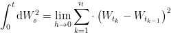
But we’ve already figured out that the right-hand side of this equation is just equal to

Differentiating both sides with respect to time gives another important stochastic identity

The Quadratic Variation of Time
Time too has a quadratic variation. Imagine the time interval ![[0,t]](https://s0.wp.com/latex.php?latex=%5B0%2Ct%5D++&bg=FFFFFF&fg=000000&s=0&c=20201002)
![[t]_t = \lim\limits_{n\rightarrow\infty}\displaystyle\sum_{i=1}^n \left(t_{i+1} - t_i\right)^2](https://s0.wp.com/latex.php?latex=%5Bt%5D_t+%3D+%5Clim%5Climits_%7Bn%5Crightarrow%5Cinfty%7D%5Cdisplaystyle%5Csum_%7Bi%3D1%7D%5En+%5Cleft%28t_%7Bi%2B1%7D+-+t_i%5Cright%29%5E2++&bg=FFFFFF&fg=000000&s=0&c=20201002)
Since time is determined by the start and end points and further by the fact that we’ve partitioned it in to 
![[0,1]](https://s0.wp.com/latex.php?latex=%5B0%2C1%5D++&bg=FFFFFF&fg=000000&s=0&c=20201002)


![[t]_t = \lim\limits_{n\rightarrow\infty}\displaystyle\sum_{i=1}^n \left(\frac{t}{n}\right)^2](https://s0.wp.com/latex.php?latex=%5Bt%5D_t+%3D+%5Clim%5Climits_%7Bn%5Crightarrow%5Cinfty%7D%5Cdisplaystyle%5Csum_%7Bi%3D1%7D%5En+%5Cleft%28%5Cfrac%7Bt%7D%7Bn%7D%5Cright%29%5E2++&bg=FFFFFF&fg=000000&s=0&c=20201002)
Now, since there are no variables indexed by 
![[t]_t = \lim\limits_{n\rightarrow\infty}\left(\frac{t}{n}\right)^2](https://s0.wp.com/latex.php?latex=%5Bt%5D_t+%3D+%5Clim%5Climits_%7Bn%5Crightarrow%5Cinfty%7D%5Cleft%28%5Cfrac%7Bt%7D%7Bn%7D%5Cright%29%5E2++&bg=FFFFFF&fg=000000&s=0&c=20201002)
which, as
![\boxed{[t]_t = 0}](https://s0.wp.com/latex.php?latex=%5Cboxed%7B%5Bt%5D_t+%3D+0%7D++&bg=FFFFFF&fg=000000&s=0&c=20201002)
We can now use the definition of an Ito integral to write
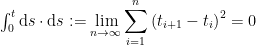
and by differentiating both sides with respect to time, obtain the result of this section:

![[Insert Equation Here]](https://s0.wp.com/latex.php?latex=%5BInsert+Equation+Here%5D++&bg=FFFFFF&fg=000000&s=0&c=20201002)

i Think sigma (t/n)^2 = (t/n)^2 sigma (1) = (t/n)^2 * n = t^2/n
yes!