Introduction
In the previous blog post we showed how an Ito calculus layer sitting on top of SageMath can produce the Black-Scholes PDE symbolically. That experiment demonstrated that symbolic manipulation of stochastic calculus is both possible and surprisingly clean once the algebra of differentials is implemented properly.
In this post we want to extend our Ito calculus layer to solve square-root processes and produce Bessel functions symbolically.
We already have a solid base where we can inject the quadratic variation term directly into the 
The implementation turns out to be surprisingly simple once the right abstraction is in place.
From Ito’s Lemma to SDE Transformations
In the previous blog post we built two core pieces of infrastructure:
- an Ito algebra class (
Ito) that automatically injects quadratic variation terms, and - a symbolic implementation of Ito’s lemma (
ito_lemma.py).
These tools allowed us to compute expressions of the form 

However, this was still slightly limited, because what we really wanted to do was to transform the SDEs themselves!
So, given an SDE for 

and a transform 

ito_lemma_scalar_state_multiW, which computes

we just need a way to take any 
Ito object representing
Let’s say we had this, then our recipe would be something like:
- compute
,
- apply the transform helper just mentioned, then
- simplify the drift, and confirm the diffusion equals
.
We have a specific, Black-Scholes-esque, 1-dimensional generator, but we want to step outside the B-S world, so we need to extend this to 2-dimensions, so for any 


Let’s get into it
New Module sde_transforms.py
Let’s create a new module called sde_transforms.py. Our first goal is to implement something which performs the Lamperti transform and then try to generalise it. Let’s import the usual stuff from typing and do our usual noinspection import of sage.all. We want the usual classes like var, SR, and diff, which we’ve used before. Finally, let’s also import our Ito class from the previous blog.
from typing import Dict, Tuple, Optional, Sequence, Union# noinspection PyUnresolvedReferencesfrom sage.all import var, SR, diff, integral, sqrt # type: ignorefrom Ito.ito_algebra import Ito
Motivation
In the previous blog, we implemented an algebra of differentials (the Ito class), and a function which specifically applies Ito’s lemma to a function. This was great at deriving PDEs but it’s not mature enough for manipulating any SDE. We must now promote the operation

to a first-class transformation of stochastic processes. Mathematically, this is called a pushforward of a diffusion. We must now stop thinking about “applying Ito’s lemma to a function
For example, suppose you have the SDE 


but conceptually what this is, is a pushforward of the diffusion under the map

where

Without this sort of abstraction, we would just end up writing special cases forever. We want to be able to handle
- Black-Scholes log transform,
- Lamperti transform (what we are working on now),
- Square-root transforms (what we want next),
- State scaling,
- Time changes,
- Girsanov transformations (the dream, end goal)
But again, all of these are just
Implementation
The simplest possible implementation is just a thin wrapper around our existing ito_lemma function. So we create a new Python module called sde_transforms.py within our Ito package:
from typing import Dict, Tuple, Optional, Sequence, Union# noinspection PyUnresolvedReferencesfrom sage.all import var, SR, diff, integral, sqrt # type: ignorefrom Ito.ito_algebra import Itofrom Ito.ito_lemma import ito_lemma_scalar_state_multiWdef sde_pushforward_scalar(phi, t, x, dX: Ito) -> Ito: """ Push forward the scalar SDE dX through the transform Y = phi(t, X). Returns dY as an Ito object: dY = mu_Y * dt + sum_i sigma_Y[i] * dW_i expressed in terms of (t, x) unless you further substitute x = phi^{-1}(y). This is literally Ito's lemma, wrapped as a semantic "SDE transform". """ return ito_lemma_scalar_state_multiW(phi, t, x, dX)def extract_sde_coeffs(dX: Ito) -> Tuple[object, Dict[int, object]]: return dX.b, dict(dX.c)def is_pure_differential(dX: Ito) -> bool: return dX.a == 0
Now, any time we want a transform (e.g. log, power, Lamperti, etc…) we don’t need to re-derive anything, we just call sde_pushforward_scalar.
This should immediately support transformations such as:
- Black-Scholes log transform,
- Lamperti transform (tested next!),
- Power transforms,
- State Scaling, and
- Time Changes
since all of these are just 
The Lamperti Transform
The Lamperti transform is supposed to eliminate state-dependent diffusion. How? Well, consider the Lamperti transform defines the following, along with its integral:

The transformed process, in general terms, 

In other words, the randomness becomes normalised. Let’s see how…
Start with the general SDE

and apply Ito’s lemma to 

Substituting the original SDE back in, and using 

OK, let’s see if this pushforward abstraction works for the Lamperti transform.
def lamperti_phi(x, sigma_x) -> object: """ Compute Lamperti transform phi(x) = ∫ 1/sigma(u) du. Returns a Sage expression (may remain unevaluated if integral is hard). """ return integral(1 / sigma_x, x)def lamperti_transform_1d(t, x, dX: Ito, dw_index: Optional[int] = None) -> Tuple[object, Ito]: """ Apply Lamperti transform to a 1D scalar SDE with a SINGLE Brownian driver: dX = mu(t,x) dt + sigma(t,x) dW Returns: (phi, dY) where Y = phi(X) and dY is the transformed SDE. Notes: - If your dX has multiple independent Brownian components, Lamperti in the "make diffusion exactly 1*dW" sense is not directly applicable without choosing a 1D driver (or doing a factor rotation). """ mu, sigmas = extract_sde_coeffs(dX) if dw_index is None: if len(sigmas) != 1: raise ValueError( f"Lamperti requires exactly one Brownian driver; got {len(sigmas)}. " f"Pass dw_index or reduce to 1D first." ) (dw_index, sigma) = next(iter(sigmas.items())) else: sigma = sigmas.get(dw_index, 0) if sigma == 0: raise ValueError(f"dw_index={dw_index} not present in dX.c") phi = lamperti_phi(x, sigma) dY = sde_pushforward_scalar(phi, t, x, dX) # Optional: nudge Sage to simplify (safe even if it doesn't change much) try: dY = Ito(dY.a, SR(dY.b).simplify_full(), {i: SR(ci).simplify_full() for i, ci in dY.c.items()}) except Exception: pass return phi, dY
Results
Here are the results.
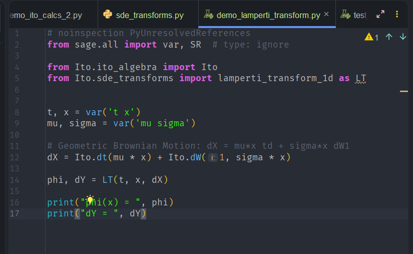
Geometric Brownian Motion
First the Geometric Brownian Motion case. We have an SDE of the form

Lamperti gives

Running the demo code produces a transformed SDE whose diffusion coefficient is exactly one:
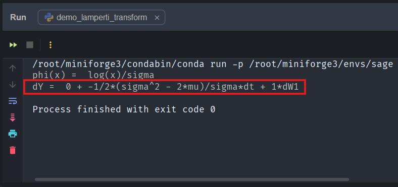
We can see that our Ito layer has correctly produced the diffusion.
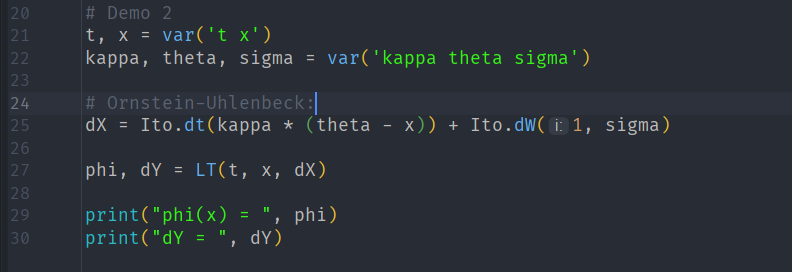
Ornstein-Uhlenbeck
For an Ornstein-Uhlenbeck (OU) process we have:

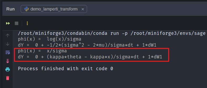
the diffusion coefficient is already constant, so Lamperti simply rescales the variable. Here, we see that the transformed diffusion coefficient is again successfully one:
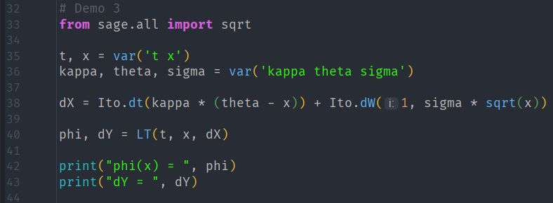
CIR Process
For the CIR process,

we have the Lamperti transforms

Here are the results
with output
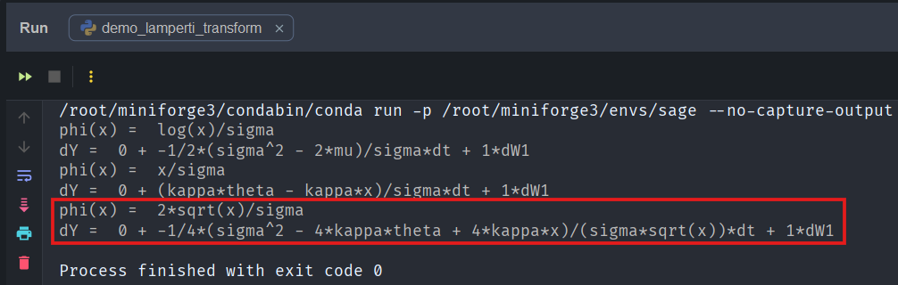
which returns

with diffusion coefficient exactly one, just as expected.
Why the Lamperti Transform Matters
The Black-Scholes model is solvable largely because the logarithm transform turns the diffusion coefficient into a constant.
The Lamperti transform generalises this idea.
Whenever an SDE has a state-dependent diffusion, such as 
Next Steps
In this post we extended our SageMath stochastic calculus layer with a generic SDE transformation framework and used it to implement the Lamperti transform.
The key conceptual shift here was to promote Ito’s lemma from a formula applied to functions, into a first-class transformation of stochastic processes.
The result of the pushforward is a new SDE with unit diffusion coefficient, which often reveals hidden structure in the process. In the case of the CIR model, the Lamperti transform exposes the connection between square-root diffusions and Bessel processes.
More importantly, the introduction of the generic pushforward operator means that we are no longer limited to isolated symbolic tricks. We now have the beginnings of a symbolic diffusion calculus where stochastic processes themselves can be transformed, analysed, and manipulated programmatically.
Road Map for Our Project
The long-term goal of this project is to perform Girsanov transformations symbolically.
Girsanov’s theorem describes how stochastic processes change under a change of probability measure. In quantitative finance this is the mechanism that converts real-world dynamics into risk-neutral dynamics, allowing derivative pricing to be expressed in terms of discounted expectations.
But before we can get there we must now spend a bit more time extending our infinitesimal generator 
References
- Øksendal, B., Stochastic Differential Equations: An Introduction with Applications.
- Shreve, S., Stochastic Calculus for Finance II.
- Karatzas, I., and Shreve, S., Brownian Motion and Stochastic Calculus.
- Revuz, D., and Yor, M., Continuous Martingales and Brownian Motion.
- Cox, J., Ingersoll, J., Ross, S., A Theory of the Term Structure of Interest Rates.
- Lamperti, J., Semi-stable stochastic processes.
- Lamperti, J., Semi-stable stochastic processes. Transactions of the American Mathematical Society (1964).
- Glasserman, P., Monte Carlo Methods in Financial Engineering.
