Infinitesimal Generators in SageMath

Introduction

In the previous two posts in this series we derived the Black–Scholes PDE using SageMath and implemented the Lamperti transform symbolically. Those exercises showed that Sage can be used not only for algebraic manipulation, but also for symbolic stochastic calculus. Just look at how well we can use SageMath to represent

The next step is to implement one of the central operators in the theory of stochastic processes: the infinitesimal generator.

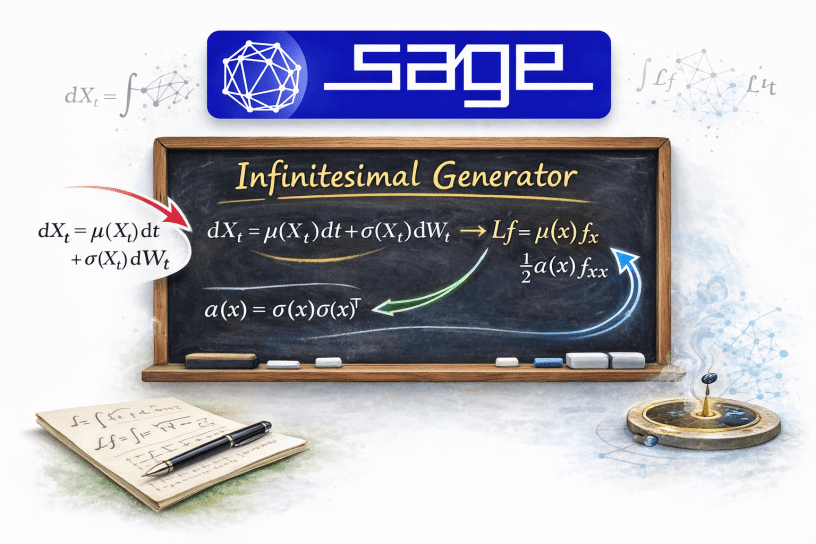
The infinitesimal generator connects stochastic differential equations (SDE) to partial differential equations (PDE). It is the mathematical object that allows us to move from a stochastic description of a process to deterministic PDEs such as the Black–Scholes equation or the Kolmogorov forward and backward equations.

In this article we implement the infinitesimal generator symbolically in SageMath and verify it against several well-known stochastic processes.

The Infinitesimal Generator

Motivation

Consider a 1-dimensional Itô diffusion

and let be the price of a derivative written on the random variable . Since is a smooth function of and of , Itô’s lemma gives

Substituting the geometric Brownian motion (GBM) dynamics back in, and using the Itô algebra result of , we get

where subscripts of functions denote partial derivatives.

Then we simply define the infinitesimal generator of the GBM process as an operator on a function :

Now we can see (by simply equating like terms) that the drift part of Itô’s lemma can be written as

and the generator leads directly to the Black-Scholes PDE. This connection is exactly what allows stochastic models to produce PDEs in the first place.

Our goal now is to build this operator symbolically in Sage and test it on a range of different diffusions.

Generators and Risk-Neutral Pricing

Let’s do a quick check to make sure that the infinitesimal generator approach will also work for martingales.

We know that under the risk-neutral measure , the discounted price process must be a -martingale, so we must have that

has zero drift (we will write a test case for this later!). Applying Itô’s lemma to the discounted process gives:

and substituting the expression for gives:

Since this is a martingale, the drift must vanish, and therefore we must again have:

which is just the Black-Scholes PDE.

So the conceptual path is:

1. Start with an SDE: ,
2. Get the infinitesimal generator: ,
3. Risk-neutral pricing says: .

For Black-Scholes, the infinitesimal generator provides the spatial differential operator in the Black-Scholes PDE, and then risk-neutral pricing adds a discounting term .

Why the Generator Matters?

The infinitesimal generator is the bridge between stochastic dynamics and PDEs.

Once the generator is available symbolically, several things become possible:

• automatic derivation of Kolmogorov equations
• verification of stochastic transformations
• proper symbolic manipulation of SDEs (our long-term goal)

In particular, it allows us to verify transformations such as the Lamperti transform by comparing generators before and after a change of variables.

More ambitiously, it provides the algebraic machinery needed for symbolic applications of Girsanov’s theorem.

Implementation

Let us create a new python module inside our Itô project, called generator.py. We will import the usual SageMath objects:

from __future__ import annotations
# noinspection PyUnresolvedReferences
from sage.all import var, SR, diff, vector, matrix  # type: ignore

The operator

will correspond to the Python code

def ito_operator_1d(f, t, x, mu, sigma):
    """
    Full Ito operator:
        (d/dt + L)[f]
    """
    ft = diff(f,t)
    return ft + generator_1d(f, x, mu, sigma)

where the generator_1d function is also defined in this module as the following spatial generator (as discussed above in the motivation):

def generator_1d(f, x, mu, sigma):
    """
    Spatial generator for 1d Ito diffusion:
        dX = mu(t,x)dt + sigma(t,x)dW
        L[f](x) = mu f_x + 1/2 sigma^2 f_xx
    """
    fx = diff(f,x)
    fxx = diff(fx,x)
    return mu * fx + SR(1) / SR(2) * (sigma ** 2) * fxx

Let us also put in some helpers:

def gradient(f, vars_):
    return vector([diff(f, v) for v in vars_])
def hessian(f, vars_):
    return matrix([[diff(f, vi, vj) for vj in vars_] for vi in vars_])

Multiple Brownian Drivers

In many models, the diffusion term is driven by several Brownian motions,

We can implement this directly in our generator.py module as another function:

def covariance_from_sigmas(sigmas: dict):
    """
    Scalar-state, multi-W case:
        a = sum_i sigma_i^2
    """
    return sum(si ** 2 for si in sigmas.values())
def generator_scalar_multiW(f, x, mu, sigmas: dict):
    """
    Generator for scalar state driven by multiple 
    independent Brownian motions.
    """
    fx = diff(f, x)
    fxx = diff(fx, x)
    a = covariance_from_sigmas(sigmas)
    return mu * fx + SR(1) / SR(2) * a * fxx

This will allow us to handle processes driven by multiple Brownian factors while still working with a single state variable.

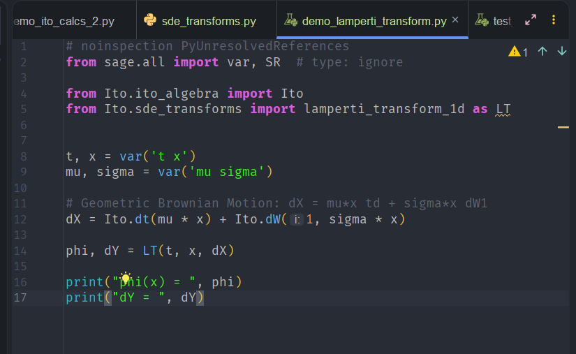
Connecting the Generator to an SDE Representation

Recall from earlier blog posts that we introduced a small symbolic algebra layer over SageMath representing Itô differentials. This way, any SDE can be now written in Python symbolically as

dX = Ito.dt(mu*x) + Ito.dW(1, sigma*x)

so that now, from this Python object, we can extract the drift and the diffusion terms and feed them into the infinitesimal generator.

Conceptually the workflow now becomes:

which will allow us to compute the generator directly from a symbolic SDE representation.

The final functions we need for the generator.py module are

def ito_operator_scalar_multiW(f, t, x, mu, sigmas: dict):
    return diff(f,t) + generator_scalar_multiW(f, x, mu, sigmas)
def generator_L_1d(f, x, mu, sigma):
    fx = diff(f,x)
    fxx = diff(fx,x)
    return mu * fx + SR(1) / SR(2) * (sigma ** 2) * fxx
def ito_operator_L_1d(f, t, x, mu, sigma):
    ft = diff(f,t)
    return ft + generator_L_1d(ft,x,mu,sigma)

and we are done and ready to test!

Results

Geometric Brownian Motion

Let us take geometric Brownian motion

the generator applied to a smooth function gives

Let us create a unittest case for this. The variables are

x, mu, sigma = var('x mu sigma')
f = x**4

We can now symbolically create the infinitesimal generator with the code

drift = mu * x
diffusion = sigma * x
Lf = generator_1d(f, x, drift, diffusion)

with an expected symbolic result of

(4 * mu + 6 * sigma**2) * x**4

Here is the demo test

# noinspection PyUnresolvedReferences
from sage.all import var, function, exp  # type: ignore
from Ito.ito_algebra import Ito
from Ito.generator import (
    gradient,
    hessian,
    generator_1d,
    ito_operator_1d,
    covariance_from_sigmas,
    generator_scalar_multiW,
    ito_operator_scalar_multiW,
)
from Ito.ito_algebra import Ito
from Ito.Igenerator import (
    generator_from_dX_1d,
    ito_operator_from_dX_1d,
    generator_from_dX_scalar_multiW,
    ito_operator_from_dX_scalar_multiW,
)
def main():
    # 1) Geometric Brownian Motion
    #      dX = mu*X dt + sigma * X dW
    x, mu, sigma = var("x mu sigma")
    # Test function
    f = x**4
    print("=== Geometric Brownian Motion Generator Demo ===")
    print("SDE: dX = mu*X dt + sigma*X dW")
    print(f"f(x) = {f}")
    print()
    fx = f.diff(x)
    fxx = fx.diff(x)
    drift = mu * x
    diffusion = sigma * x
    print(f"f_x   = {fx}")
    print(f"f_xx  = {fxx}")
    print(f"mu(x) = {drift}")
    print(f"sigma(x) = {diffusion}")
    print()
    Lf = generator_1d(f, x, drift, diffusion)
    expected = (4 * mu + 6 * sigma**2) * x**4
    print("Infinitesimal generator:")
    print("L[f] = mu(x) * f_x + (1/2) * sigma(x)**2 * f_xx")
    print()
    print(f"Symbolic output L[f] = {Lf}")
    print(f"Expected closed form = {expected}")
    print()
    check = (Lf - expected).expand().simplify_full()
    print(f"Check L[f] - expected = {check}")
    if check == 0 or getattr(check, 'is_zero', lambda: False)():
        print("Demo passed.")
    else:
        print("Demo failed.")
if __name__ == "__main__":
    main()

and here is the output

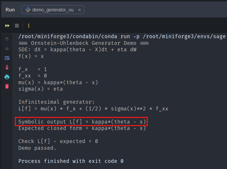
Test OU Process

The Ornstein-Uhlenbeck (OU) process is defined by the SDE

the generator applied to a smooth function , with derivatives , gives

Substituting these into the infinitesimal generator gives

which is exactly the drift term of the OU process. In other words, we see again that the generator correctly reproduces the deterministic component of the dynamics when applied simply to the identity function.

Let us create a unittest case for this. The variables are

x, kappa, theta, eta = var('x kappa theta eta')
f = x

We can now symbolically create the infinitesimal generator with the code

drift = kappa * (theta - x)
diffusion = eta
Lf = generator_1d(f, x, drift, diffusion)

with an expected symbolic result of

kappa * (theta - x)

Here is the demo test result:

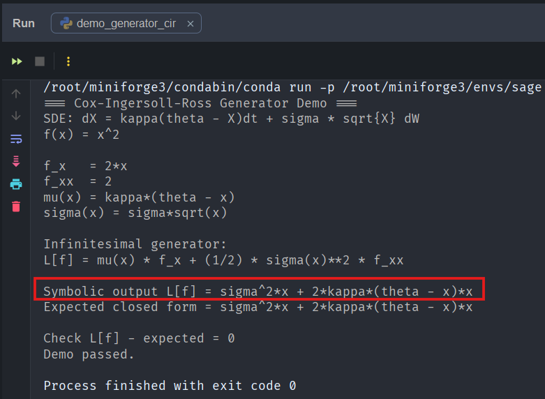
Test CIR Process

The Cox-Ingersoll-Ross (CIR) process is defined by the SDE

the generator applied to a smooth function , with derivatives , gives

Substituting these into the infinitesimal generator gives

Let us create a unittest case for this. The variables are

x, kappa, theta, sigma = var('x kappa theta sigma')
f = x**2

We can now symbolically create the infinitesimal generator with the code

drift = kappa * (theta - x)
diffusion = sigma * sqrt(x)
Lf = generator_1d(f, x, drift, diffusion)

with an expected symbolic result of

2 * kappa * x * (theta - x) + sigma**2 * x

Here is the demo test result:

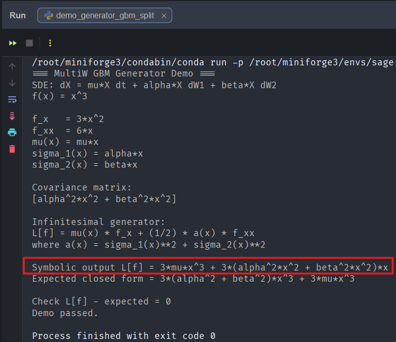
Test 2-dimensional Geometric Brownian Motion

For a 2-dimensional GBM we have the simplified SDE

with scalar-state diffusion covariance

Note that we really actually have a -covariance matrix

which collapses to the scalar:

Since, and , we get

So for a scalar state process with split GBM processes, the infinitesimal generator becomes

Now let’s take the smooth function , with derivatives and , we get

Let us create a unittest case for this. The variables are

x, mu, alpha, beta = var("x mu alpha beta")
f = x**3

We can now symbolically create the infinitesimal generator with the code

drift = mu * x
sigma1 = alpha * x
sigma2 = beta * x
covariance_matrix = matrix([[sigma1**2 + sigma2**2]])
covariance_scalar = covariance_matrix[0,0]
Lf = generator_scalar_multiW(f, x, drift, {1: sigma1, 2: sigma2})

with an expected symbolic result of

3 * mu * x**3 + 3 * (alpha**2 + beta**2) * x**3

Here is the demo test result:

Conclusion

In this post we implemented the infinitesimal generator of an Itô diffusion symbolically in SageMath and verified it against several well-known stochastic processes.

Together with the Lamperti transform implemented earlier, this forms the foundation of a symbolic stochastic calculus toolkit.

The next step will be to extend the generator to vector-valued diffusions, allowing us to work with multi-dimensional models such as stochastic volatility systems and affine term-structure models.

From there, we move closer to the ultimate goal of this project: performing transformations such as Girsanov’s theorem symbolically within SageMath.

References

1. Øksendal, B. (2003). Stochastic Differential Equations.
2. Karatzas & Shreve (1991). Brownian Motion and Stochastic Calculus.

Appendix

Python Module generator.py

from __future__ import annotations
# noinspection PyUnresolvedReferences
from sage.all import var, SR, diff, vector, matrix  # type: ignore
def gradient(f, vars_):
    return vector([diff(f, v) for v in vars_])
def hessian(f, vars_):
    return matrix([[diff(f, vi, vj) for vj in vars_] for vi in vars_])
def generator_1d(f, x, mu, sigma):
    """
    Spatial generator for 1d Ito diffusion:
        dX = mu(t,x)dt + sigma(t,x)dW
        L[f](x) = mu f_x + 1/2 sigma^2 f_xx
    """
    fx = diff(f,x)
    fxx = diff(fx,x)
    return mu * fx + SR(1) / SR(2) * (sigma ** 2) * fxx
def ito_operator_1d(f, t, x, mu, sigma):
    """
    Full Ito operator:
        (d/dt + L)[f]
    """
    ft = diff(f,t)
    return ft + generator_1d(ft, x, mu, sigma)
def covariance_from_sigmas(sigmas: dict):
    """
    Scalar-state, multi-W case:
        a = sum_i sigma_i^2
    """
    return sum(si ** 2 for si in sigmas.values())
def generator_scalar_multiW(f, x, mu, sigmas: dict):
    """
    Generator for scalar state driven by multiple
    independent Brownian motions.
    """
    fx = diff(f, x)
    fxx = diff(fx, x)
    a = covariance_from_sigmas(sigmas)
    return mu * fx + SR(1) / SR(2) * a * fxx
def ito_operator_scalar_multiW(f, t, x, mu, sigmas: dict):
    return diff(f,t) + generator_scalar_multiW(f, x, mu, sigmas)
def generator_L_1d(f, x, mu, sigma):
    fx = diff(f,x)
    fxx = diff(fx,x)
    return mu * fx + SR(1) / SR(2) * (sigma ** 2) * fxx
def ito_operator_L_1d(f, t, x, mu, sigma):
    ft = diff(f,t)
    return ft + generator_L_1d(ft,x,mu,sigma)