Kolmogorov Equations in SageMath

In the previous blog posts we have built an Ito Layer over SageMath in Python, implemented the Lamperti transform, and an infinitesimal generator. This mean that we can create stochastic differential equation (SDE) objects using python commands such as

dS = Ito.dt(mu * S) + Ito.dW(1, sigma * S)

to represent

which tells us how the state moves locally. But in practice, nobody cares about the infinitesimal increment itself… everyone cares about how the expectation of some payoff functional changes as we move slightly through time? In other words, everyone cares about the conditional expectation:

We know this because in quant finance it’s called the option price, in particle filtering it’s called the prediction, and in physics it’s called the observable. Let’s just say it’s a big deal.

But how does this extend from all our work on the infinitesimal generator? We built an operator object , in Python, which acts on functions of a random variable in ways like:

The truth is, this generator has always told us the instantaneous rate of change of expectations, we just didn’t know it! How? Well, it hinges on the Markov property of the stochastic process , and we’ll derive this a little later in the blog.

Let’s go back and look at the expectation of a payoff functional at some infinitesimally small time earlier. If we do this, the change that we observe must be governed by the generator – because as we will see, it’s part of the definition!

When you push that argument to the limit $latex\varepsilon\rightarrow 0$, the result is

This is called the backward Kolmogorov equation.

The recipe thus becomes something like this: start with an SDE (e.g. geometric Brownian motion). Find the infinitesimal generator, plug it in to the backward Kolmogorov equation, attach the terminal boundary condition, out pops the pricing PDE.

Now, we could also evolve expectations forward in time. That is, take what we know now, like some current state probability transition density, and evolve it forward in time. In a similar way, another pricing PDE should pop out (spoiler alert, it will be the adjoint PDE of the one we get when going backwards in time).

The infinitesimal generator contains all the information we need about the stochastic dynamics, and from it we obtain two complementary evolution-in-time equations:

• the backward Kolmogorov equation, which evolves expectations of future quantities backward in time to current time, and
• the forward Kolmogorov equation (a.k.a the Fokker-Planck equation), which evolves probability densities (of the current state) forward in time.

The Infinitesimal Generator and the Expectation

The big question which needs answering is this: How does the infinitesimal generator define the instantaneous rate of change of expectations? This seems to be the real link between what we did in the previous blog, and this one. Without a good understanding of this step, the next implementation will feel a bit too much like magic.

To see how the two link, let us consider a (continuous-time) Markov process and some test functional . Define the expectation as per usual,

This function tells you the expected value of if the process starts at .

Now introduce the operator

This operator is called the Markov semigroup; and they just propagate expectations forward in time. And yes! the semigroup property follows from the Markov property and the tower rule for conditional expectations. So the “Markov semigroup” label here is just that family of operators that propagate expectations forward in time, and the infinitesimal generator is just the time derivative of this operator family at .

Recall our infinitesimal generator,

That fraction there is literally the time derivative:

So by definition, the infinitesimal generator is actually just the derivative of the expectation! So it is indeed part of the definition. In other words, the generator is nothing more than the deterministic first-order part of the Itô expansion after taking expectations.

So the ideas are:

• Expectations (as functions obtained after integrating against a probability measure) propagate forward via action of the Markov semigroup,
  • Elements of the semigroup pull (payoff) functionals backward (through a change of parameter , and
  • Adjoint elements push probability densities forward,
• The infinitesimal generator is defined now as the derivative of that semigroup at ,
• For diffusions, Ito’s lemma lets you compute the generator explicitly as,

This means that the backward Kolmogorov equation becomes pretty obvious! Say, if

then the semigroup representation is

Differentiate this with respect to time and the generator pops out:

So the infinitesimal generator is not just “some operator associated with the SDE“. No, it is literally the derivative of the expectation operator that pushes functionals (of the random variable) forward in time.

Implementation of the Kolmogorov Equations

The starting point is what we already have, which is the infinitesimal generator

where .

Then, we know we have the Kolmogorov equations:

• Backward Kolmogorov for is
  • , with terminal boundary condition .
• Forward Kolmogorov for $p(t,x)$ is the adjoint
  • 

where the adjoint is

In Python, we would want functions that look like this:

backward_kolmogorov(u, t, state_vars, drift, diffusion)
forward_kolmogorov(p, t, state_vars, drift, diffusion)
formal_adjoint_applied(phi, t, state_vars, drift, diffusion)

where:

• state_vars is [x] or [x, y, ...]
• drift is [mu1, mu2, ...]
• diffusion is either
  • a scalar or list of factors, or
  • a covariance matrix

Let us create a new Python module called kolmogorov.py.

from __future__ import annotations
# noinspection PyUnresolvedReferences
from sage.all import var, SR, diff, matrix  # type: ignore
def ensure_list(x):
    return x if isinstance(x, list) else [x]
def covariance_from_diffusion(diffusion, n):
    """
    Convert diffusion specification into covariance matrix a = sigma sigma^T.
    Supported:
      - scalar expression for 1D
      - list of expressions for diagonal independent factors in 1D or componentwise
      - Sage matrix interpreted directly as covariance matrix if shape is n x n
      - rectangular sigma matrix, converted to sigma * sigma.transpose()
    """
    if hasattr(diffusion, "nrows") and hasattr(diffusion, "ncols"):
        if diffusion.nrows() == n and diffusion.ncols() == n:
            return diffusion
        return diffusion * diffusion.transpose()
    if n==1:
        diffs = ensure_list(diffusion)
        return matrix(SR, 1, 1, [sum(g**2 for g in diffs)])
    diffs = ensure_list(diffusion)
    if len(diffs) != n:
        raise ValueError("For multi-dimensional state, diffusion must be an n x n marix, or a length-n diagonal list!")
    sigma = matrix(SR, n, n, 0)
    for i in range(n):
        sigma[i, i] = diffs[i]
    return sigma * sigma.transpose()
def generator(f, state_vars, drift, diffusion):
    """
    Apply infinitesimal generator L to a test functional f.
    L[f](x) = sum_i b_i d_i f + 0.5 sum_{i,j} a_{ij} d_{ij} f
    :param f:
    :param state_vars:
    :param drift:
    :param diffusion:
    :return:
    """
    xs = ensure_list(state_vars)
    bs = ensure_list(drift)
    n = len(xs)
    if len(bs) != n:
        raise ValueError("Drift length must match number of state variables!")
    a = covariance_from_diffusion(diffusion, n)
    first_order = sum(bs[i] * diff(f, xs[i]) for i in range(n))
    second_order = sum(
        a[i, j] * diff(f, xs[i], xs[j])
        for i in range(n)
        for j in range(n)
    ) / 2
    return first_order + second_order
def formal_adjoint_applied(phi, state_vars, drift, diffusion):
    """
    Apply the formal adjoint L* to phi
    L*phi = -sum_i d_i(b_i phi) + 1/2 sum_{i,j} d_{ij}(a_{ij} phi)
    :param phi:
    :param state_vars:
    :param drift:
    :param diffusion:
    :return:
    """
    xs = ensure_list(state_vars)
    bs = ensure_list(drift)
    n = len(xs)
    if len(bs) != n:
        raise ValueError("Drift length must match number of state variables!")
    a = covariance_from_diffusion(diffusion, n)
    drift_term = -sum(diff(bs[i] * phi, xs[i]) for i in range(n))
    diffusion_term = sum(
        diff(a[i, j] * phi, xs[i], xs[j])
        for i in range(n)
        for j in range(n)
    ) / 2
    return drift_term + diffusion_term
def backward_kolmogorov(u, t, state_vars, drift, diffusion, simplify_result=True):
    """
    Returns the Backward Kolmogorov PDE expression:
    u_t + L u
    :param u:
    :param t:
    :param state_vars:
    :param drift:
    :param diffusion:
    :param simplify_result:
    :return:
    """
    expr = diff(u, t) + generator(u, state_vars, drift, diffusion)
    return expr.simplify_full() if simplify_result else expr
def forward_kolmogorov(p, t, state_vars, drift, diffusion, simplify_result=True):
    """
    Returns the Forward Kolmogorov PDE expression:
    p_t - L* p
    :param p:
    :param t:
    :param state_vars:
    :param drift:
    :param diffusion:
    :param simplify_result:
    :return:
    """
    expr = diff(p, t) - formal_adjoint_applied(p, state_vars, drift, diffusion)
    return expr.simplify_full() if simplify_result else expr

Methods of Kolmogorov.py

The kolmogorov.py module sits one level above the Itô layer. Its job is to take a drift and diffusion specification for an Itô diffusion, build the associated second-order differential operator, and then assemble the backward and forward Kolmogorov equations symbolically.

ensure_list(x)

This is a small utility function that normalises inputs. If x is already a list, it is returned unchanged. Otherwise it is wrapped into a one-element list.

This lets the rest of the module accept either scalar inputs, such as a single state variable $x$x, or vector inputs, such as , without duplicating logic everywhere. It is not glamorous, but it stops the rest of the code from becoming annoying.

covariance_from_diffusion(diffusion, n)

This method converts the user’s diffusion specification into the covariance matrix

It supports several cases.

If the diffusion input is already a Sage matrix, then:

• if it is an matrix, it is interpreted directly as the covariance matrix ,
• otherwise it is treated as a diffusion loading matrix , and the method returns .

If the state is one-dimensional, the method also allows a scalar diffusion coefficient or a list of scalar diffusion coefficients. In that case it returns

which corresponds to multiple independent Brownian factors driving the same scalar state variable.

For a multi-dimensional state, the method also accepts a list of length , interpreted as diagonal diffusion loadings. It builds the diagonal matrix

and returns .

So this method is really the adapter between several convenient user-facing diffusion formats and the single mathematical object the Kolmogorov equations actually want: the covariance matrix .

generator(f, state_vars, drift, diffusion)

This applies the infinitesimal generator to a test function .

Given state variables ​, drift vector , and diffusion specification, it computes

Internally, the method first converts the diffusion input into the covariance matrix , then constructs:

• the first-order drift term,
• the second-order diffusion term.

This is the core operator of the module. Everything else in kolmogorov.py is built from it. Conceptually, this is the object that governs the local evolution of conditional expectations.

formal_adjoint_applied(phi, state_vars, drift, diffusion)

This applies the formal adjoint to a function . The formula used is

Where the generator acts naturally on test functions or payoff functions, the adjoint acts naturally on densities. This is the operator that appears in the forward Kolmogorov, or Fokker-Planck, equation.

So if generator(...) is the expectation-side operator, then formal_adjoint_applied(...) is the density-side operator. Same diffusion, same dynamics, opposite side of the duality.

backward_kolmogorov(u, t, state_vars, drift, diffusion, simplify_result=True)

This constructs the symbolic expression for the backward Kolmogorov equation:

If the returned expression is set equal to zero, this gives the PDE

This is the equation satisfied by conditional expectation functionals of the form

The method simply computes the time derivative , adds the generator applied to , and optionally simplifies the result with Sage’s simplify_full().

This is the method you use when moving from an SDE to a pricing-style or expectation-style PDE.

forward_kolmogorov(p, t, state_vars, drift, diffusion, simplify_result=True)

This method constructs the symbolic expression for the forward Kolmogorov equation:

If the returned expression is set equal to zero, this gives

This is the PDE governing the evolution of the density of the diffusion. In one dimension it becomes the familiar Fokker-Planck form:

So while the backward equation evolves observables or payoff functionals, the forward equation evolves probability mass. This method makes that density evolution symbolic and explicit.

Summary of Module Methods

The design of kolmogorov.py is deliberately compact:

• covariance_from_diffusion(...) converts user diffusion input into the covariance matrix,
• generator(...) builds the infinitesimal generator ,
• formal_adjoint_applied(...) builds the adjoint operator ,
• backward_kolmogorov(...) returns ,
• forward_kolmogorov(...) returns .

Taken together, these methods form the bridge from symbolic Itô calculus to symbolic PDE construction. That is exactly why this module matters. It is the point where an SDE stops being just a stochastic differential equation and starts becoming an operator-theoretic object with both backward and forward evolution equations attached to it, because apparently one equation was not enough for humanity.

Demonstration

Let us now run a simple demo.

Suppose the underlying asset follows geometric Brownian motion

and suppose we want the value of the European put option with payoff at maturity .

The quantity we want SageMath/Python to compute is the conditional expectation:

which is exactly the object we introduced earlier in this blog.

Now, according to the backward Kolmogorov equation, the value functional must satisfy

where is the infinitesimal generator of the diffusion; which for GBM is .

Let us now use our SageMath implementation of Ito.kolmogorov to construct this PDE symbolically:

from sage.all import *
from kolmogorov import backward_kolmogorov
t, T, S, K, mu, sigma = var('t T S K mu sigma')
u = function('u')(t, S)
pde = backward_kolmogorov(
    u,
    t,
    S,
    mu * S,
    sigma * S
)
payoff = max_symbolic(K - S, 0)
print("Backward PDE:")
print(pde == 0)
print("Terminal condition:")
print(u.subs(t=T) == payoff)

This produces the output

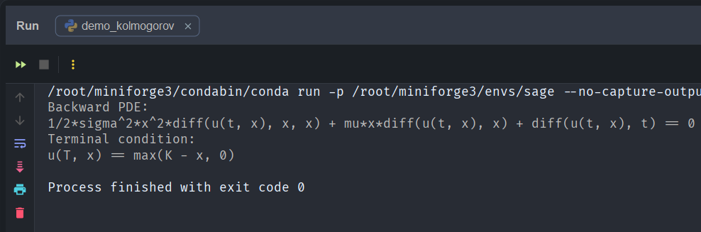
and this is exactly the backward Kolmogorov PDE associated with geometric Brownian motion.

So with nothing more than:

• the stochastic differential equation governing the dynamics of the underlying asset, and
• the terminal payoff functional

we can get SageMath to symbolically derive the PDE governing the option value.

From Kolmogorov to Black-Scholes

The Black-Scholes equation is just a backward Kolmogorov equation under a change of measure. Let’s find out why.

So at this point in the demonstration we have obtained this:

with terminal condition , but this is not yet the Black-Scholes PDE! We now go through the usual steps of changing the measure from the physical to the risk-neutral one.

Recall that a discounted asset price must be a martingale. Thus, must be a martingale.

Under Girsanov’s theorem, it is well known that we change the Brownian motion via

where

So let’s substitute this back! Start with

Replace :

Expand:

Substitute :

The drift changed: , and the diffusion term did not change. The generator has the same structure, and it changes in exactly the same places. So under it is

Then, when we define the discounted option value

the backward Kolmogorov equation becomes

and substituting the generator gives the correct Black-Scholes option pricing PDE:

In other words, the Black-Scholes equation is simply the risk-neutral backward Kolmogorov equation for geometric Brownian motion.

Lognormal Demo

We can drive the fact home by running the following demo:

# noinspection PyUnresolvedReferences
from sage.all import sqrt, pi, exp, var, log, function  # type: ignore
import Ito.kolmogorov as Kolmogorov
t, S, S0, mu, sigma = var('t S S0 mu sigma', domain='positive')
p = function('p')(t, S)
pde = Kolmogorov.forward_kolmogorov(p, t, S, mu * S, sigma * S)
density = (
    1 / (S * sigma * sqrt(2 * pi * t))
    * exp(
        -(
            log(S / S0) - (mu - sigma**2 / 2) * t
        )**2 / (2 * sigma**2 * t)
    )
)
residual = Kolmogorov.forward_kolmogorov(
    density, t, S, mu * S, sigma * S
).simplify_full()
print("Forward PDE:")
print(pde == 0)
print("\nGBM lognormal density:")
print(density)
print("\nResidual after direct substitution:")
print(residual)
print("\nVerified:")
print(residual == 0)

with output:

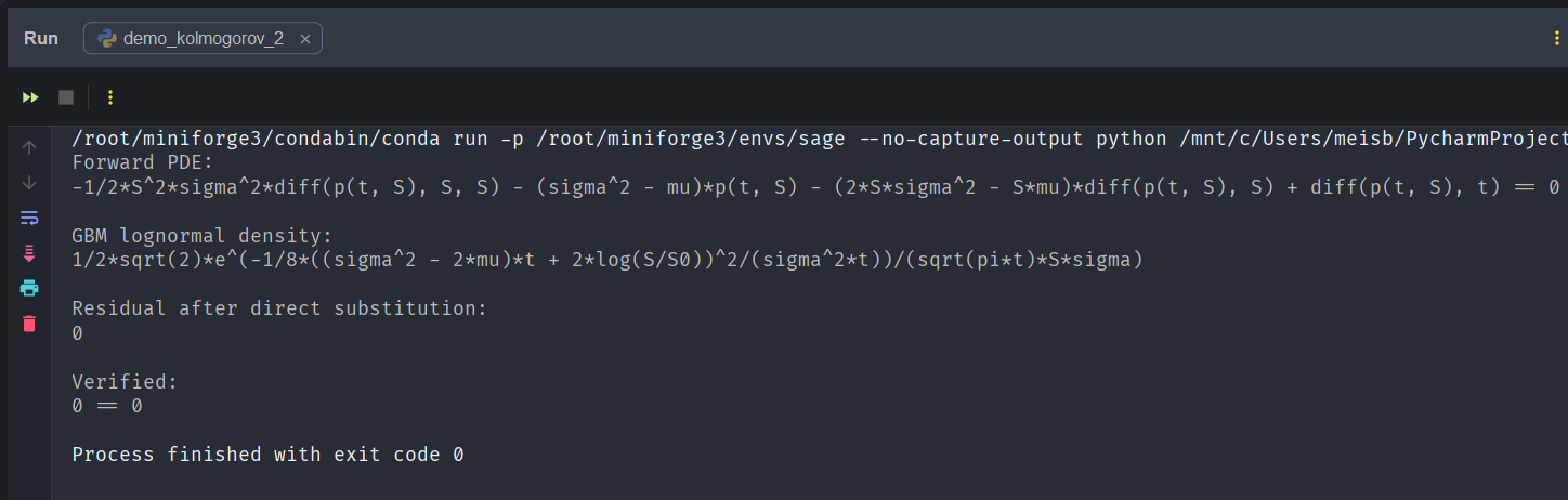
To make the forward Kolmogorov equation less abstract, we can verify directly that the known lognormal transition density of geometric Brownian motion satisfies it. Starting from the GBM SDE, our SageMath implementation constructs the forward PDE symbolically. We then substitute the closed-form lognormal density into the PDE residual and simplify. The result is zero, confirming that the forward Kolmogorov equation is exactly the PDE governing the evolution of the GBM transition density.

Conclusion

This demonstration shows that we can begin with an SDE

and a choice of terminal boundary condition (i.e. option payoff at expiry)

Then define the value functional

Now, SageMath and our Ito layer does not really “solve the SDE“; instead, it really computes first the infinitesimal generator

and then uses the backward Kolmogorov equation to know that must satisfy

so that our Ito layer will substitute in, and out pops the backward PDE:

So this goes: SDE + Payoff Generator Backward PDE Pricing PDE.

The Black-Scholes PDE requires one more modelling step because it is not written with the physical drift , it is written under the risk-neutral measure, where the underlying asset price drift becomes .

Next Up

In the next post we will begin exploring how these symbolic tools connect to

• the Feynman-Kac theorem
• risk-neutral pricing
• and eventually symbolic Girsanov transformations

which will allow us to manipulate stochastic models directly at the level of their generators.

References

1. https://en.wikipedia.org/wiki/Kolmogorov_backward_equations_(diffusion)
2. https://en.wikipedia.org/wiki/Fokker%E2%80%93Planck_equation

Appendix

Module Kolmogorov.py

from __future__ import annotations
# noinspection PyUnresolvedReferences
from sage.all import var, SR, diff, matrix  # type: ignore
def ensure_list(x):
    return x if isinstance(x, list) else [x]
def covariance_from_diffusion(diffusion, n):
    """
    Convert diffusion specification into covariance matrix a = sigma sigma^T.
    Supported:
      - scalar expression for 1D
      - list of expressions for diagonal independent factors in 1D or componentwise
      - Sage matrix interpreted directly as covariance matrix if shape is n x n
      - rectangular sigma matrix, converted to sigma * sigma.transpose()
    """
    if hasattr(diffusion, "nrows") and hasattr(diffusion, "ncols"):
        if diffusion.nrows() == n and diffusion.ncols() == n:
            return diffusion
        return diffusion * diffusion.transpose()
    if n==1:
        diffs = ensure_list(diffusion)
        return matrix(SR, 1, 1, [sum(g**2 for g in diffs)])
    diffs = ensure_list(diffusion)
    if len(diffs) != n:
        raise ValueError("For multi-dimensional state, diffusion must be an n x n marix, or a length-n diagonal list!")
    sigma = matrix(SR, n, n, 0)
    for i in range(n):
        sigma[i, i] = diffs[i]
    return sigma * sigma.transpose()
def generator(f, state_vars, drift, diffusion):
    """
    Apply infinitesimal generator L to a test functional f.
    L[f](x) = sum_i b_i d_i f + 0.5 sum_{i,j} a_{ij} d_{ij} f
    :param f:
    :param state_vars:
    :param drift:
    :param diffusion:
    :return:
    """
    xs = ensure_list(state_vars)
    bs = ensure_list(drift)
    n = len(xs)
    if len(bs) != n:
        raise ValueError("Drift length must match number of state variables!")
    a = covariance_from_diffusion(diffusion, n)
    first_order = sum(bs[i] * diff(f, xs[i]) for i in range(n))
    second_order = sum(
        a[i, j] * diff(f, xs[i], xs[j])
        for i in range(n)
        for j in range(n)
    ) / 2
    return first_order + second_order
def formal_adjoint_applied(phi, state_vars, drift, diffusion):
    """
    Apply the formal adjoint L* to phi
    L*phi = -sum_i d_i(b_i phi) + 1/2 sum_{i,j} d_{ij}(a_{ij} phi)
    :param phi:
    :param state_vars:
    :param drift:
    :param diffusion:
    :return:
    """
    xs = ensure_list(state_vars)
    bs = ensure_list(drift)
    n = len(xs)
    if len(bs) != n:
        raise ValueError("Drift length must match number of state variables!")
    a = covariance_from_diffusion(diffusion, n)
    drift_term = -sum(diff(bs[i] * phi, xs[i]) for i in range(n))
    diffusion_term = sum(
        diff(a[i, j] * phi, xs[i], xs[j])
        for i in range(n)
        for j in range(n)
    ) / 2
    return drift_term + diffusion_term
def backward_kolmogorov(u, t, state_vars, drift, diffusion, simplify_result=True):
    """
    Returns the Backward Kolmogorov PDE expression:
    u_t + L u
    :param u:
    :param t:
    :param state_vars:
    :param drift:
    :param diffusion:
    :param simplify_result:
    :return:
    """
    expr = diff(u, t) + generator(u, state_vars, drift, diffusion)
    return expr.simplify_full() if simplify_result else expr
def forward_kolmogorov(p, t, state_vars, drift, diffusion, simplify_result=True):
    """
    Returns the Forward Kolmogorov PDE expression:
    p_t - L* p
    :param p:
    :param t:
    :param state_vars:
    :param drift:
    :param diffusion:
    :param simplify_result:
    :return:
    """
    expr = diff(p, t) - formal_adjoint_applied(p, state_vars, drift, diffusion)
    return expr.simplify_full() if simplify_result else expr

Module test_kolmogorov.py

import unittest
# noinspection PyUnresolvedReferences
from sage.all import var, function, matrix, SR, diff  # type: ignore
import Ito.kolmogorov as Kolmogorov
class TestKolmogorov1D(unittest.TestCase):
    def test_generator_gbm_1d(self):
        x, mu, sigma = var('x mu sigma')
        f = function('f')(x)
        a = matrix(SR, [[sigma**2 * x**2]])
        actual = Kolmogorov.generator(f, x, mu * x, a)
        expected = mu * x * diff(f, x) + (sigma**2 * x**2 / 2) * diff(f, x, x)
        self.assertEqual((actual - expected).simplify_full(), 0)
    def test_backward_gbm_1d(self):
        t, x, mu, sigma = var('t x mu sigma')
        u = function('u')(t, x)
        a = matrix(SR, [[sigma ** 2 * x ** 2]])
        actual = Kolmogorov.backward_kolmogorov(u, t, x, mu * x, a)
        expected = diff(u, t) + mu * x * diff(u, x) + (sigma ** 2 * x ** 2 / 2) * diff(u, x, x)
        self.assertEqual((actual - expected).simplify_full(), 0)
    def test_forward_gbm_1d(self):
        t, x, mu, sigma = var('t x mu sigma')
        p = function('p')(t, x)
        a = matrix(SR, [[sigma ** 2 * x ** 2]])
        actual = Kolmogorov.forward_kolmogorov(p, t, x, mu * x, a)
        expected = diff(p, t) + diff(mu * x * p, x) - diff(sigma ** 2 * x ** 2 * p, x, x) / 2
        self.assertEqual((actual - expected).simplify_full(), 0)
if __name__ == '__main__':
    unittest.main()