Introduction
In the previous blog we introduced the Kolmogorov Forward and Backward equations and showed how they arise from the infinitesimal generator of a SDE. That exercise demonstrated that once the stochastic dynamics are expressed symbolically, SageMath can manipulate them in much the same way as classical calculus. In this post we extend that idea one step further. Instead of stopping at the Kolmogorov equations, we now show how the same symbolic representation of an SDE can be used to automatically construct the exponential martingale associated with the process. This object plays a central role in stochastic calculus because it forms the density process that enables changes of probability measure, ultimately leading to Girsanov’s theorem.
In this blog we aim to be able to write, with minimal effort, some Python code that builds an SDE with an interface which looks like this:
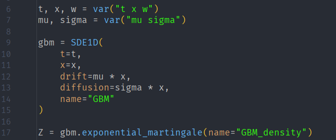
and for it to produce a result that looks like this:
Before we get to the code, let’s motivate why we need a 1-dimensional SDE class object.
Motivation
The derivation in the previous post relied on manually specifying the stochastic dynamics. In practice we would like some higher-level abstraction in our code, namely, some Python class object that represents a (1-dimensional) SDE which knows how to manipulate its own symbolic structure (using our Ito layer) in some automatic fashion.
The goal of this blog is therefore to introduce a symbolic framework centered around the SDE1D class object. This object represents a 1-dimensional Ito diffusion of the form:

Once instantiated, this object will expose several useful symbolic operations, namely:
- construct the infinitesimal generator,
- apply Ito’s lemma to a transformation of the process, and
- compute the Lamperti transform that converts the diffusion coefficient into
.
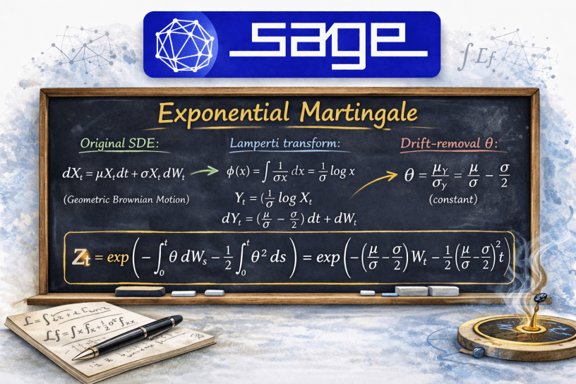
The Lamperti transform plays a crucial role within this class object. We define it as

then the transform stochastic process takes the form of a unit-diffusion with drift 

Once in this form, a natural quantity appears:

This drift-removal ratio is precisely what appears in the stochastic exponential:

Now, processes of this form are known as exponential martingales and they play a key role in the context of changes in probability measure.
The aim of this blog is therefore to demonstrate that our SDE1D class object can automatically derive the ingredients needed to construct this exponential martingale. In other words, our object can symbolically derive the density process implied by the stochastic dynamics. This will serve as the bridge between this and the next topic, which will be on measure changes and Girsanov’s theorem.
Implementation
For this blog, only one new Python module is implemented, sde.py, which introduces a small symbolic class object for 1-dimensional Ito diffusions. In this section we will discuss how it is implemented.
The core object is the SDE1D class, which represents a stochastic differential equation (SDE) of the form
and it holds the data needed to specify it at any given time. This class stores the symbolic data:
- time variable
t, - state variable
x, - drift function
drift, and - diffusion function
diffusion
Once instantiated, the object exposes several methods that allow symbolic manipulation of the stochastic dynamics. In particular, the class provides methods to
- construct the Itô differential representation of the SDE,
- apply the infinitesimal generator to a test function,
- apply Itô’s lemma to a transformation of the process, and
- compute the Lamperti transform, which converts the diffusion coefficient to unity.
The Lamperti transform is implemented by pushing the SDE through a scalar transformation

which will produce a unit-diffusion.
The SDE1D class
dataclass(frozen=True)class SDE1D: """ Symbolic 1D Itô SDE dX_t = drift(t, x) dt + diffusion(t, x) dW_{dw_index} This class is the user-facing object for your symbolic stochastic layer. It wraps the existing Ito algebra and transform utilities into a cleaner API. Parameters ---------- t : Sage symbol Time variable. x : Sage symbol State variable. drift : Sage expression Drift coefficient mu(t, x). diffusion : Sage expression Diffusion coefficient sigma(t, x). dw_index : int Brownian motion index. Default is 1. name : Optional[str] Optional label for display/debugging. """ t: object x: object drift: object diffusion: object dw_index: int = 1 name: Optional[str] = None def differential(self) -> Ito: """ Return the Ito differential representation of the SDE: dX = drift*dt + diffusion*dW_{dw_index} """ return Ito.dt(self.drift) + Ito.dW(self.dw_index, self.diffusion) def dX(self) -> Ito: """ Alias for differential(), since this is the notation people actually want. """ return self.differential() def coeffs(self) -> Dict[str, Any]: """ Return a structured dictionary of the SDE coefficients. """ return { "t": self.t, "x": self.x, "drift": self.drift, "diffusion": self.diffusion, "dw_index": self.dw_index, "name": self.name, } def generator(self, f, simplify_result: bool = True): """ Apply the infinitesimal generator to a test function f(x) or f(t,x): L[f] = mu * f_x + 1/2 sigma^2 * f_xx """ fx = diff(f, self.x) fxx = diff(fx, self.x) expr = self.drift * fx + SR(1) / SR(2) * (self.diffusion ** 2) * fxx if simplify_result: try: return SR(expr).simplify_full() except Exception: return expr return expr def ito_operator(self, f, simplify_result: bool = True): """ Apply the full Itô operator: (∂/∂t + L)[f] """ ft = diff(f, self.t) expr = ft + self.generator(f, simplify_result=False) if simplify_result: try: return SR(expr).simplify_full() except Exception: return expr return expr def pushforward(self, phi, simplify_result: bool = True) -> Ito: """ Push forward the SDE through a scalar transform Y = phi(t, x) returning dY as an Ito object. """ dY = sde_pushforward_scalar(phi, self.t, self.x, self.dX()) if simplify_result: try: return Ito( dY.a, SR(dY.b).simplify_full(), {i: SR(ci).simplify_full() for i, ci in dY.c.items()} ) except Exception: return dY return dY def transformed_coeffs(self, phi, simplify_result: bool = True) -> Dict[str, Any]: """ Push forward through Y = phi(t,x) and return extracted coefficients. Returns ------- dict { "phi": phi, "dY": Ito(...), "drift": mu_Y, "diffusions": {i: sigma_i^Y} } """ dY = self.pushforward(phi, simplify_result=simplify_result) mu_Y, sigmas_Y = extract_sde_coeffs(dY) if simplify_result: try: mu_Y = SR(mu_Y).simplify_full() except Exception: pass try: sigmas_Y = {i: SR(si).simplify_full() for i, si in sigmas_Y.items()} except Exception: pass return { "phi": phi, "dY": dY, "drift": mu_Y, "diffusions": sigmas_Y, } def lamperti(self, simplify_result: bool = True) -> Dict[str, Any]: """ Apply the Lamperti transform to the SDE. For a 1D one-factor diffusion, this computes phi(x) = ∫ (1 / sigma(x)) dx and returns the transformed SDE dY. Returns ------- dict { "phi": phi, "dY": Ito(...), "drift": mu_Y, "diffusion": sigma_Y } """ phi, dY = lamperti_transform_1d( self.t, self.x, self.dX(), dw_index=self.dw_index ) mu_Y, sigmas_Y = extract_sde_coeffs(dY) sigma_Y = sigmas_Y.get(self.dw_index, 0) if simplify_result: try: phi = SR(phi).simplify_full() except Exception: pass try: mu_Y = SR(mu_Y).simplify_full() except Exception: pass try: sigma_Y = SR(sigma_Y).simplify_full() except Exception: pass return { "phi": phi, "dY": dY, "drift": mu_Y, "diffusion": sigma_Y, } def drift_removal_theta(self, simplify_result: bool = True): """ Compute the drift-removal ratio from the Lamperti-transformed SDE: theta = mu_Y / sigma_Y In the standard Lamperti case, sigma_Y = 1, so theta = mu_Y. This is the natural bridge to exponential martingales and later Girsanov. """ data = self.lamperti(simplify_result=False) mu_Y = data["drift"] sigma_Y = data["diffusion"] if sigma_Y == 0: raise ValueError("Lamperti-transformed diffusion vanished; cannot form theta = mu_Y / sigma_Y.") theta = mu_Y / sigma_Y if simplify_result: try: return SR(theta).simplify_full() except Exception: return theta return theta def exponential_martingale(self, theta=None, name=None, simplify_result=True): if theta is None: return ExponentialMartingale1D.from_lamperti( self, name=name, simplify_result=simplify_result ) return ExponentialMartingale1D.from_theta( self, theta=theta, name=name, simplify_result=simplify_result )
The ExponentialMartingale1D Class
The same module also introduces a second symbolic class object called ExponentialMartingale1D, whose purpose is to represent the stochastic exponential associated with a 1-dimensional Ito diffusion.
The object is intentionally not another Ito diffusion, but rather designed to be a symbolic wrapper around the formal expression:
where 
The class stores four main pieces of information:
- the underlying
SDE1Dobject, - the symbolic expression for the drift-removal
- the Brownian driver index, and
- an optional name for display purposes.
There are two class constructors. The first, from_theta, allows the object to be created directly from a user-supplied drift-removal parameter from_lamperti, derives SDE1D object by calling the drift_removal_theta method. In this way, the stochastic exponential can either be specified explicitly or discovered symbolically from the SDE itself.
Once constructed, the class provides several convenience methods. The theta() method returns the stored symbolic coefficient, while formal() and to_latex() produce string and LaTeX representations of the stochastic exponential. These are useful when printing the resulting density process to the console or embedding it directly into the blog output.
For the special case in which constant_theta_closed_form, which collapses the stochastic exponential into the explicit expression:

A second helper, verify_constant_theta, then checks symbolically that this expression satisfies

which is the backward Kolmogorov equation associated with zero Itô drift. This gives us a direct symbolic verification that, in the constant-
Taken together, the ExponentialMartingale1D class provides the final layer required to move from a symbolic SDE to its associated density process. It is this object that makes the bridge from the Lamperti-transformed dynamics to exponential martingales explicit in code.
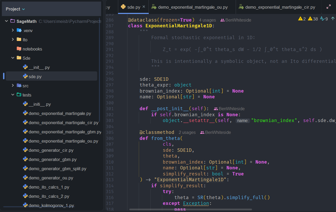
dataclass(frozen=True)class ExponentialMartingale1D: """ Formal stochastic exponential in 1D: Z_t = exp( -∫_0^t theta_s dW - 1/2 ∫_0^t theta_s^2 ds ) This is intentionally a symbolic object, not an Ito differential. """ sde: SDE1D theta_expr: object brownian_index: Optional[int] = None name: Optional[str] = None def __post_init__(self): if self.brownian_index is None: object.__setattr__(self, "brownian_index", self.sde.dw_index) classmethod def from_theta( cls, sde: SDE1D, theta, brownian_index: Optional[int] = None, name: Optional[str] = None, simplify_result: bool = True ) -> "ExponentialMartingale1D": if simplify_result: try: theta = SR(theta).simplify_full() except Exception: pass return cls( sde=sde, theta_expr=theta, brownian_index=brownian_index if brownian_index is not None else sde.dw_index, name=name ) classmethod def from_lamperti( cls, sde: SDE1D, name: Optional[str] = None, simplify_result: bool = True ) -> "ExponentialMartingale1D": theta = sde.drift_removal_theta(simplify_result=simplify_result) return cls.from_theta( sde=sde, theta=theta, brownian_index=sde.dw_index, name=name, simplify_result=simplify_result ) def theta(self, simplify_result: bool = True): theta = self.theta_expr if simplify_result: try: return SR(theta).simplify_full() except Exception: pass return theta def ito_integral_str(self) -> str: return f"∫_0^{self.sde.t} ({self.theta()}) dW{self.brownian_index}" def dt_integral_str(self) -> str: return f"∫_0^{self.sde.t} ({self.theta()})^2 ds" def formal(self) -> str: return (f"exp(-({self.ito_integral_str()}) - 1/2*({self.dt_integral_str()}))") def to_latex(self) -> str: theta_ltx = latex(self.theta()) t_ltx = latex(self.sde.t) i = self.brownian_index return ( r"\exp\!\left(" + rf"-\int_0^{t_ltx} {theta_ltx}\, dW_{{{i}}}" + rf"- \frac{{1}}{{2}}\int_0^{t_ltx} ({theta_ltx})^2\, ds" + r"\right)" ) def constant_theta_closed_form(self, w, simplify_result: bool = True): """ If theta is constant, return the explicit closed form Z(t,w) = exp(-theta*w - 1/2 theta^2 t) where w is a symbolic Brownian/state variable. """ theta = self.theta(simplify_result=False) if theta is None: raise ValueError( "theta is None. Build or derive the exponential martingale " "before calling constant_theta_closed_form()." ) expr = exp(-theta * w - SR(1) / SR(2) * theta**2 * self.sde.t) if simplify_result: try: return SR(expr).simplify_full() except Exception: return expr return expr def verify_constant_theta(self, w, simplify_result: bool = True) -> Dict[str, Any]: """ Verify, in the constant-theta case, that Z_t + 1/2 Z_ww = 0 i.e. the backward heat equation associated with zero Ito drift. """ Z = self.constant_theta_closed_form(w, simplify_result=False) Z_t = diff(Z, self.sde.t) Z_ww = diff(Z, w, 2) residual = Z_t + SR(1) / SR(2) * Z_ww if simplify_result: try: Z = SR(Z).simplify_full() except Exception: pass try: Z_t = SR(Z_t).simplify_full() except Exception: pass try: Z_ww = SR(Z_ww).simplify_full() except Exception: pass try: residual = SR(residual).simplify_full() except Exception: pass return { "Z": Z, "Z_t": Z_t, "Z_ww": Z_ww, "residual": residual, }
Now on to Results.
Results
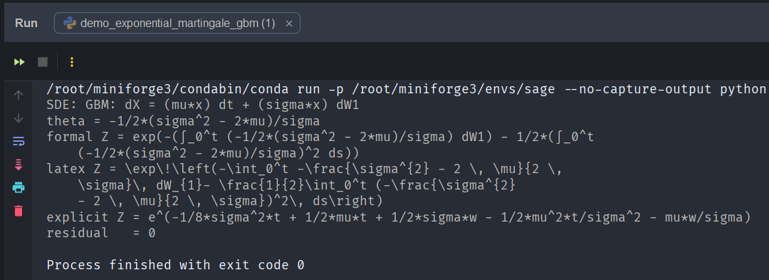
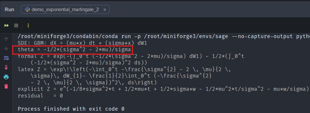
Geometric Brownian Motion
For our first test we will implement geometric Brownian motion (GBM) with our new class object.
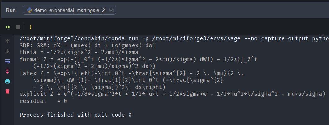
For GBM, we start with

The Lamperti transform is

So if the transformed process is

then Ito’s lemma gives a transformed SDE of the form

and the diffusion coefficient has been normalised to unity, the exact purpose of the Lamperti transform. This means our

Since this value is constant, the stochastic exponential simplifies considerably. Substituting it into the general form of the exponential martingale gives

which is the exponential martingale associated with geometric Brownian motion.
Now, because the drift-removal ratio verify_constant_theta, which symbolically confirms that this expression satisfies the following backward Kolmogorov equation corresponding to Brownian motion with zero drift:

In other words, our symbolic engine verifies directly that the resulting process has zero drift, confirming that the stochastic exponential is indeed a martingale:
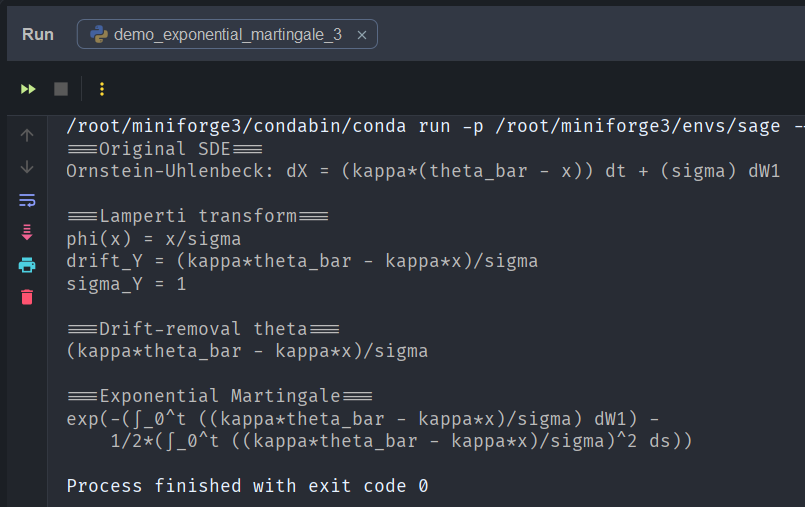
Ornstein-Uhlenbeck
Now lets test the SDE1D class object on the Ornstein-Uhlenbeck (OU) process, which has the form

Unlike geometric Brownian motion, the diffusion coefficient is already constant. This means the Lamperti transform is particularly simple:

So we define the transformed process as

then Ito’s lemma gives:

and again the Lamperti transform has successfully converted the OU process into a unit-diffusion process, but now with a drift that remains state-dependent.
From the transformed SDE we can therefore simply read off the drift-removal ratio:

or equivalently in the 

which matches exactly what our code produces (see below figure).
Substituting this drift-removal coefficient into the universal form of the stochastic exponential gives the formal exponential martingale

and, unlike the GBM case, we do not obtain a closed-form expression here because the drift-removal ratio is not constant. For that reason, this is not a case where we can apply the helper function verify_constant_theta. Instead, the significance of the OU test is that it shows that our symbolic framework is already capable of deriving a state-dependent drift-removal coefficient and substituting it directly into the formal stochastic exponential.
So even in the mean-reverting OU setting, the Python console output is giving us the density process implied by the stochastic dynamics:
Cox-Ross-Ingersoll
Now let’s try the 1-dimensional Cox-Ingersoll-Ross (CIR) stochastic process with our new class object.
For CIR, we start with

The Lamperti transform is

So if

then Ito’s lemma gives a transformed SDE of the form

which means our

Transforming back to the 

…and we get a match with our code:
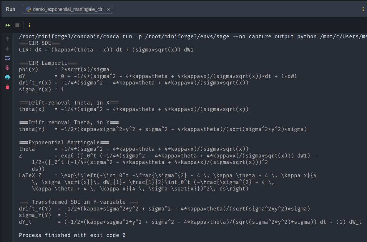
So we have a match on the Lamperti transform, and the drift-removal theta in both 
sigma_Y(x) = 1 output.
Direct substitution into the stochastic exponential (which always has the same structural form) gives us the formal exponential martingale:
![\displaystyle Z_t = \exp\left(-\int_0^t \left[\frac{4\kappa\theta - \sigma^2}{2\sigma^2 Y_s} - \frac{1}{2}\kappa Y_s\right]dW_s - \frac{1}{2}\int_0^t \left[\frac{4\kappa\theta - \sigma^2}{2\sigma^2 Y_s} - \frac{1}{2}\kappa Y_s\right]^2 ds\right)](https://s0.wp.com/latex.php?latex=%5Cdisplaystyle+Z_t+%3D+%5Cexp%5Cleft%28-%5Cint_0%5Et+%5Cleft%5B%5Cfrac%7B4%5Ckappa%5Ctheta+-+%5Csigma%5E2%7D%7B2%5Csigma%5E2+Y_s%7D+-+%5Cfrac%7B1%7D%7B2%7D%5Ckappa+Y_s%5Cright%5DdW_s+-+%5Cfrac%7B1%7D%7B2%7D%5Cint_0%5Et+%5Cleft%5B%5Cfrac%7B4%5Ckappa%5Ctheta+-+%5Csigma%5E2%7D%7B2%5Csigma%5E2+Y_s%7D+-+%5Cfrac%7B1%7D%7B2%7D%5Ckappa+Y_s%5Cright%5D%5E2+ds%5Cright%29&bg=%23ffffff&fg=%23111111&s=0&c=20201002)
Unlike the GBM test case, we do not want to run verify_constant_theta(w) here because this 
However, this means that our 1-d SDE class object, and its methods, are capable of deriving a state-dependent drift-removal coefficient! In the end, what we have is that this object:
- Computes the Lamperti transform,
- Extracts the transformed drift,
- Computes the drift-removal coefficient, then
- Substitutes this drift-removal coefficient directly into the formula for the stochastic exponential.
If nothing else, this means the output we automatically get in the console is the density process implied by the SDE.
Next Steps
Since we can now automatically derive symbolically the density process implied by the SDE, we should now be able to multiply the probability measure by the exponential martingale 
Being able to manipulate probability densities in this fashion brings us one step closer to Girsanov.
Conclusion
We have now built the first real bridge between our symbolic Ito layer and the measure-change machinery that will eventually give us Girsanov. We can now start with an SDE, say geometric Brownian motion:
gbm = SDE1D(t, x, drift, diffusion)
which represents
and the SDE class object knows how to compute the infinitesimal generator. It does this by application of the Lamperti transform, so it computes:

It then pushes the SDE object through this transformation to get

thus converting the GBM SDE into a unit-diffusion process with constant drift.
The SDE object then knows how to extract the drift and define

and since 

which can be seen here:
This is precisely the coefficient needed to remove the drift via a stochastic exponential.
The SDE class object then goes further and constructs the exponential martingale:

Because
The SDE class object method verify_constant_theta then checks that this equation satisfies the backward Kolmogorov equation associated with Brownian motion:
where now subscripts indicate partial derivatives, which is this line here:
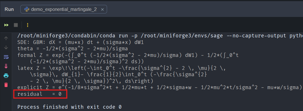
and it has confirmed that the stochastic exponential has zero drift, thus proving that it is now a martingale in this setting.
To summarise:
- Take an SDE and compute the Lamperti Transform,
- Extract the drift-removal ration
- Construct the corresponding exponential martingale,
- Verify that the resulting process has zero drift.
References
- Øksendal, B. (2003). Stochastic Differential Equations.
- Karatzas & Shreve (1991). Brownian Motion and Stochastic Calculus.
