It’s not that quantum computers are faster or smaller than classical computers that makes them different. Rather, quantum computers operate on a set of principles that are completely different to the principles used by classical computers. But what are these principles? I think this is a pretty good place to start before we delve in to quantum computing.
So in this article we will take a look at the principles underpinning classical computer science. Why these principles came about and what they solve and allow us to do. We will look in to a very important conjecture that allows us to cast literally any problem that a human mind can conceive in to a simple mathematical model (thanks to the genius of Alan Turing). Finally, we will take a look in to classical logic gates that allow computation to occur, setting the stage to look at one of the first defining features of a quantum computer.
Turing Machines
There is a guiding principle that allows us to answer questions about classical computers. Questions like: “What can and cannot be computed?” can be simplified by the Church-Turing thesis. While this conjecture has not been proven (and even borders on the realm of philosophy) it is certainly a very useful thing to believe is true. In other words we assume it is a definition of what is and what is not computable, thus allowing us to focus our efforts.
To understand the Church-Turing thesis one needs to know first what a Turing Machine is, since the thesis states that computability (as understood by a human calculating an answer to a problem) is fundamentally linked to whether or not that same problem can be computed by a Turing machine. This means that to answer the question: “Can this be computed?” we no longer need to go off and test the computation on every conceivable computer – we just need to test it on a Turing machine.
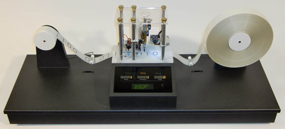
A Turing Machine is really the simplest way to represent a thing which calculates stuff – in the sense that it achieves an answer to a problem as posed by a human, and the answer itself is recognisable by that human (or controller). Simply put, a Turing Machine consists of an infinitely long piece of tape upon which is listed an infinitely long sequence of letters (including a special letter known as zero which represents “do nothing”). There is also a device which reads the letters (called a “head”) and can write new letters; it can also move up and down the tape, one letter at a time. Finally, there is a set of instructions that tells the head to either delete or create a new letter on the tape, move the head up or down, or do something at a particular site. Sounds simple enough.

The concept of a Turing Machine was a breakthrough to computer science because it was the first time in history that we were able to represent our ability to solve a problem by manipulating symbols in terms of a physical apparatus (although they are theoretical models). In a sense, a Turing Machine approaches a problem in a very similar way to how a human would with a pen and paper.
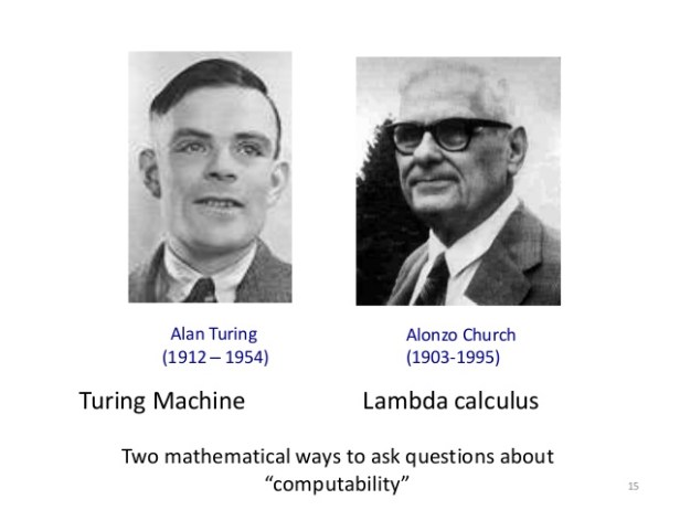
There are two important results pertaining to a Turing Machine as described above and first thought of by Alan Turing in 1936. First, there now must exist what is known as a universal Turing Machine which is capable of simulating the behaviour of any other Turing Machine (and therefore, any other computing machine that anyone could think of), simply by modifying the initial configuration of the infinitely long tape. Turing said of this machine in his 1936 paper:
It is possible to invent a single machine which can be used to compute any computable sequence. If this machine is supplied with a tape on the beginning of which is written the standard description of an action table of some other computing machine then it will compute the same sequence.
Second, and even more remarkable, is that this universal Turing machine need not be very complicated at all! In fact, it would only need a tape with just 4 symbols and a head with just 7 states (e.g. an example of a state is the instruction to move up or down, delete or create new, etc… Remember that the head must always have the halting state – that state which instructs the machine to stop calculating.), this is the celebrated Minksy Machine discovered by (the now cryogenically frozen) Marvin Minsky back in 1962. Other small universal Turing machines exist, for example Claude Shannon‘s example from 1956 that had just two symbols (but the number of states where undefined).
The Halting Problem
A natural question arises at this point: “Given any problem that a human can think up, and assuming a suitable algorithm is known to provide a solution to that problem, is it possible to determine if the Turing machine will ever finish calculating?“. I.e. can you know beforehand if the final state (and thus, the solution) will be reached? This is known as the Halting Problem and was proven by Turing himself in 1936 to be undecidable, i.e. it is impossible to design a Turing machine to determine if another will halt or not.
This leads to perhaps the most important question of computers by today’s standard: “How long will a computation take to complete?“. Obviously the answer is infinitely long if the problem is undecidable. If the problem is decidable then the time it takes to complete the computation is found by counting the number of elementary operations performed by the algorithm to arrive at the solution. This is known as Time Complexity.
Polynomial Time
The Cobham-Edmonds conjecture states that any computation is feasible if they can be computed in something called polynomial time. This is to say that there exists an algorithm that (given an tape of letters a certain amount long, say 10) can produce an answer within 10 to the power of x seconds, where x is a number associated to the problem type (not a particular instance of the problem). In other words, the time it takes to compute an answer is always less than this upper bound. Ideally, for problem types that has, say x = 2, then if the input is 10 bits of information long, then the solution will take 10^2=100 seconds to compute. Realistically though, x is usually very small.
Such problems are said to belong to the complexity class P (standing for Polynomial), and, adhering to the concept of a universal Turing Machine: if a human provides an algorithm that solves a problem in polynomial time (with respect to the size of the input and the type of problem) then this algorithm will always run in polynomial time on any computer. Likewise, a problem that requires exponential time on any computer will require exponential time on every computer.
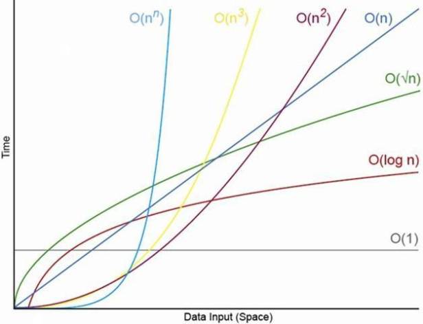
The division between polynomial and exponential problems is also convenient because it corresponds to our intuition of what is a efficient or inefficient algorithm. An algorithm that requires n operations is certainly faster than one which requires n^2 operations (both polynomial), but both are much, much faster that one which requires 2^n operations (exponential). In the exponential case, one does not need n to be very large before the problem is considered impossible. Thus, exponential algorithms are considered intractable.
For this reason one is frequently concerned with being able to distinguish polynomial-time algorithms from exponential-time algorithms.
Non-Deterministic Turing Machines
Interestingly, a Turing Machine operating a polynomial-time algorithm can be made in to an exponential-time algorithm simply by introducing one additional property: that at every operational step, the machine replicates itself in to a different state (i.e. it performs a different operation from the operation set) and then continues operating on the same input string. Pretty soon there are an exponential number of Turing Machines. The machine solves the problem only if at least one of the machines finds a solution. But no matter how it does it, it will have still performed an exponential number of operations. This is known as a non-deterministic Turing Machine. How does this non-deterministic machine know which action it should take? Unless you actually physically replicate the Turing Machine at every junction, you could simply “role a dice” allowing chance or some sort of probability distribution drive the choice, until eventually a solution is found. Once a solution is found, it is easy to imagine then that only one path is taken (the one and only path leading to the solution), ignore the rest, and proclaim that the machine is the “luckiest possible guesser“! The other way to imagine it is that the machine as a computation tree where if it least one branch of the tree halts with a solution then we say that the machine has found a solution.
Are Quantum Computers Non-Deterministic Turing Machines?
No, not quite. First of all, Turing Machines are not physical computers they are mathematical models. But what about Quantum Turing Machines? Do they exist. Yes, they do. They are different to Non-Deterministic Turing Machines, fundamentally and we will get to the difference soon.
Logic Gates
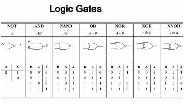
Every computation can be viewed as some operation that takes an input string (like a tape consisting of ones and zeroes) and returns an output string (of ones and zeroes) representing the answer to some problem. A Logic Gate is the simplest operation that a machine can perform on a single bit of information. For example, the NOT gate works like this: If a=1 then NOT(a)=0. If a=0 then NOT(a)=1. You could theoretically add a NOT state to the head of a Turing Machine so that when it read a 1 on the input tape, the head would delete the 1 and write a 0 there instead. There are other logic gates too! For example, if a=1 and b=1 then AND(a,b)=1 but if either a=0 or b=0 then AND(a,b)=0. There is also the OR gate which says that if a=1 or b=1 then OR(a,b)=1, otherwise if a=0 and b=0 then OR(a,b)=0. To each of these there is the alternative denial gates NAND and NOR; plus the exclusive gates XOR and XNOR. Finally there is the unique gate COPY which takes an input and creates two of the same as an output, thus COPY(a)=a a.
Once we have a set of logic gates we can apply a sequence of them, one after the other, to produce quite complicated operations. This is fundamentally the definition of an algorithm.
This set of gates (AND, NOT the alternatives and exclusives, plus COPY) form what is known as a universal set (or functional completeness) such that any problem can be computed. Furthermore it satisfies the Church-Turing thesis.
The Church-Turing Thesis
The Church-Turing thesis states that a problem is computable by an algorithm if and only if it is computable by a universal set of logic gates on a Turing Machine. Often the term “computable” is replaced by the term “computable function“. Interestingly, before this term was defined, mathematicians often used the informal term effectively calculable to describe operations that were computable by pencil-and-paper methods.
Effectively what this conjecture says (and if you choose to believe it or not – believing it certainly does ensure some interesting things to study!) is that the notion of computable (as what a human does) is the same as running input tape through the head of a Turing Machine that results in a decisive solution.
From here the entire subject of Computer Science was born, and without it we would still be guessing at how to effectively solve problems by testing algorithms on every conceivable computer system. Even though the conjecture is strongly believed but as yet unproven, that has not stopped scientists from checking every now and again. So far, every single conceivable model for a computer has been tested against the conjecture and every single one of them has found to be equivalent to a Turing Machine – that’s a pretty good track record!
A good way to think of the Church-Turing thesis is that whenever you pick some intuitive notion of computable the resulting model of computation is either equivalent to a Turing Machine or strictly weaker – and thus not worth studying. So you might as well study the Turing Machine.
Summary
In this first article on quantum computing we went back to basics and looked at what it means for a problem to be computable by a machine. We introduced the notion of a Turing Machine as a construct for the simplest type of computing apparatus possible. We encountered problems that could not be solved (e.g. the Halting Problem) forcing us to consider only those which had solutions. This led us to the concept of Time Complexity by asking “how long does it take?” and we found that some computations could be solved faster than others by applying an upper bound based on the size of the input and the class of problem – thus separating algorithms that can be solved in polynomial time versus those requiring exponential time.
We looked a deterministic versus non-deterministic Turing Machines by considering Turing Machines that exponentially duplicated in other to test more than one state at every junction. We got agonisingly close to our first definition of a quantum computer but realised that they are more than just non-deterministic Turing Machines.
Then we looked at the simplest kind of operation a Turing Machine can do and realised that we only need 3 to compute every single kind of conceivable operation, namely the NOT, AND and COPY gates (plus their alternatives and exclusives).
Finally, by considering the above, we could describe the Church-Turing thesis which underpins the majority of modern computer science.
Next
In this next article we will look more closely at these classical logic gates and consider the concept of reversibility and discover an important linkage between classical logic and thermodynamics! We will encounter truth tables and penalty functions for our logic gates and consider the concept of garbage. A new gate will be considered, the controlled-NOT gate (or CNOT gate) and this will be our first jump in to quantum computing.
