Understanding the Phase Kickback Trick in Quantum Computing

Introduction

In the previous article we looked at the generalised Hadamard transform and how it has this neat effect of placing the qubit basis state label into the exponent of the coefficient (the phase) of a transformed basis state:

$\displaystyle H^{\otimes n}|x\rangle = \frac{1}{\sqrt{2^n}} \sum_{z=0}^{2^n - 1} (-1)^{x\cdot z} |z\rangle$

Now that we know how information gets placed in to the phase of a qubit, what can we do with it?

In this article we are going to look at the Phase Kickback Trick (PKT), which is a trick that utilises this ability to place information in to the phase of a qubit, but also how we can transfer phase information from one qubit to another by using controlled quantum gates (or controlled unitaries).

Origins of the PKT appear in the Quantum algorithms – revisited (1998) paper of Cleve, Ekert, Macchiavello & Mosca, although according to John Watrous, the authors credit Alain Tapp (the same author of the Brassard-Høyer-Tapp algorithm of 1997) for independently discovering the trick. David Deutsch came very close to discovering it while publishing his eponymous algorithm in 1992, but didn’t actually use it.

Binary Representations

To be able to understand the PKT we first need to get familiar with binary representations of integers.

Let’s use the integer $a=3$ as our starting example.

We now ask: what is this in binary?

The short answer is that it is: $11$ .

The slightly longer answer is that it is a length-2 bitstring – the term “bitstring” is to say that it is a string of symbols from the alphabet of bits (i.e. $0$ ‘s and $1$ ‘s) but, in general, they could be any symbol from any 2-letter alphabet, which we denote $\sigma_2$ .

Someone a little more familiar with binary might say that it is also a length-3 bitstring! After all, $11$ canbe re-written trivially as $011$ by simply appending a redundant $0$ symbol at the beginning.

Then, eadem ratione it’s also the length-4 bitstring $0011$ – with two redundant leading $0$ ‘s.

We can keep going and say that the integer $a=3$ is equal to $0\dots 011$ by padding-out (as they say) as many leading zeros as we wish. The more leading zeroes we append, the more qubits we need to add to our quantum register, and the higher dimension of our problem.

So, for now, let us work with just one leading zero so that $a = 3 = 011$ and hence, we have $n=3$ qubits and thus the dimension of our system is $N = 2^n = 2^3 = 8$ . Recall, the dimension is eight because qubits are two-state systems (i.e. the alphabet has two letters) and have 2 degrees of freedom, hence why we raise two to the power of 3, and not one.

For each of the three symbol slots in the 3-dimensional binary representation $011$ we could instead do away with any specific reference to an alphabet of symbols and just write $a_1 a_2 a_3$ (indexed by the natural numbers) as the binary representation of the integer $a = 3$ . In this case we would have $a_1 = 0$ and $a_2 = a_3 = 1$ .

But keep in mind that for a arbitrary integer $0 \leq a \leq 7$ the binary expansion would be $a_1 a_2 a_3$ , i.e. just 3 digits long, as we prescribed. The second we go above $7$ we need a new symbol slot, an extra qubit, an extra dimension.

Binary Representations

What we need now is a formula for the binary expansion given any length $n$ that we desire. Thinking about this for a minute or two we realise that

$\displaystyle a = 3 = 0 + 2 + 1$

Why did we bother with the zero in that sum? Well, there is good reason and it has to do with the number of qubits we chose initially. Since we are working with 3 qubits we want 3 summands. This is because we can re-write the above sum as

$\displaystyle a = 3 = 0 + 2 + 1 = (2^2 \cdot 0) + (2^1 \cdot 2) + (2^0 \cdot 1)$

This is the standard binary representation of an integer $a$ . Those exponents $2^2,\, 2^1,\, 2^0$ are like coefficients. Indeed for any integer $0 \leq a \leq 7$ , we would have

$\displaystyle a = (2^2 \cdot a_1) + (2^1 \cdot a_2) + (2^0 \cdot a_3)$

which generalises to any integer $a \in \mathbb{Z}$ ,

$\displaystyle a = 2^{n-1}\cdot a_1 + 2^{n-2}\cdot a_2 + \cdots + 2^1 \cdot a_{n-1} + 2^0 \cdot a_n$

where $a_i \in \{0,1\}$ .

We can go one step further and write this sum more compactly as

$\displaystyle a = \sum_{j=1}^{n} 2^{n-j} a_j$

With a dimension/string-length $n=3$ , we can plug in an integer, say $a=3$ . in to this formula to get:

$\displaystyle 3 = \sum_{j=1}^{3} 2^{n-j}a_j = 2^{3-1} a_1 + 2^{3-2} a_2 + 2^{3-3} a_3 = 4a_1 + 2a_2 + a_3$

So we get the ( $n=3$ ) equation for $a = 3$ to be:

$\displaystyle \sum_{j=1}^{3} 2^{n-j}a_j = 4a_1 + 2a_2 + a_3 = 3$

which has a solution (in the group $(\mathbb{Z}_2,\cdot)$ ) given by

$\displaystyle a_1 = 0, \quad\quad\quad\quad a_2 = a_3 = 1$

Thus, according to the formula, the ( $n=3$ ) binary expansion of the integer $3$ is:

$\displaystyle a_1a_2a_3 = 011$

and that’s how you do it.

Why Binary Structure Matters for Phase Kickback

Since the generalised Hadamard outputs amplitudes of the form

$\omega^{xz} = e^{2\pi i (xz) / 2^n}$

the product $xz$ must be evaluated using binary multiplication. And this is crucial! When you multiply by an integer $x$ , the resuling phase breaks into a product of phases, each corresponding to each qubit $x_j$ . Thus, with an integer with binary representation such as,

$x = \displaystyle\sum_{j=0}^{n-1} x_j 2^j$

we have that

$\displaystyle\frac{xz}{2^n} = \displaystyle\sum_{j=0}^{n-1} x_j\frac{2^j z}{2^n} = \displaystyle\sum_{j=0}^{n-1} x_j\frac{y}{2^{n-j}}$

resulting in

$e^{2\pi i (xz) / 2^n} = \displaystyle\prod_{j=0}^{n-1}e^{2\pi i x_j z / 2^{n-j}}$

And since each $x_j \in \{0,1\}$ , each bit simply toggles whether a phase rotation is applied or not.

The Controlled-U Gate

As mentioned briefly in the introduction, we aim to be able to transfer information from a target qubit to the phase of a control qubit. To do this we will need a controlled unitary operator.

Unitary Operators and Eigenstates

Consider a unitary operator $U$ . We have already seen in a previous article that this has an intimate relationship with a given quantum state $|\psi\rangle$ , a qubit $|x\rangle$ and the phase, which we will denote as $\lambda$ for now, but will take on a more specific form in just a moment. The reason for this intimate relationship is due to the eigenvalue-eigenvector (EE) problem, click on this link to refresh yourself on the origins of this problem before continuing, or read how this is used with qubits in the previous article.

One of the first things we can say about the unitary $U$ is that it could share an eigenvalue $\lambda$ with the quantum state $|\psi\rangle$ . If it does, then we say that the quantum state $|\psi\rangle$ is an eigenstate of the unitary operator $U$ , and you can write down the EE problem quite simply as:

$\displaystyle U|\psi\rangle = \lambda|\psi\rangle$

This is the definition of an eigenstate – it must be defined with an operator and an associated eigenvalue.

The EE-problem for a unitary operator and a quantum state is to say that: applying the unitary operator $U$ to the target qubit $|\psi\rangle$ does not change its state, but only changes its phase – which takes the form of the associated eigenvalue $\lambda$ – this is literally reading off the above equation. And since $U$ is unitary, all its eigenvalues satisfy $|\lambda| = 1$ , so they can all be written as a pure phase $\lambda = e^{i\theta},\,\theta\in\mathbb{R}$ .

In the language of linear algebra this is nothing but a square matrix multiplied by a column vector (ket) equalling another scaled column vector, where the amount of scaling that occurs is just the eigenvalue $\lambda$ .

The question is: can we take the phase (the eigenvalue) and somehow apply it to another qubit? Can we transfer phase information from one qubit to another?

While not immediately obvious, the answer is: Yes.

In what is to come, we need to keep in mind our assumptions:

We have chosen a particular unitary operator $U$ that works with a qubit in such a way that the qubit is an eigenvector of $U$ with an eigenvalue $\lambda$ . The assumption here is that we have this linear EE problem; and
We aim to be able to take this eigenvalue/phase and actually do something with it, namely: somehow encode the phase onto another qubit (called the target qubit).

A Little Preview

To set the scene for what is to come, observe the following neat property of a unitary $U$ acting on a quantum state $|\psi\rangle$ .

From the property of the eigenvalues we already have $U|\psi\rangle = e^{i\theta}|\psi\rangle$ . The controlled version of the unitary must act as

$|0\rangle|\psi\rangle \rightarrow |0\rangle|\psi\rangle$
$|1\rangle|\psi\rangle \rightarrow |1\rangle e^{i\theta}|\psi\rangle$

which results in a combined state

$\alpha|0\rangle|\psi\rangle + \beta|1\rangle|\psi\rangle e^{i\theta}$

and, importanly, the state can be factored out!

$|\psi\rangle\left(\alpha|0\rangle + \beta e^{i\theta} |1\rangle\right)$

The target is unchanged and the phase appears on the control qubit! Exactly as we want.

Note that we have just shown how the phase kickback works automatically with a control qubit, a target qubit (initialised in an eigenstate of some unitary), and a controlled version of that unitary. However, many quantum algorithms also use an Oracle, so in the next section we will present the phase kickback trick as being packaged together with an Oracle (even though technically it is not required).

The Phase Kickback Trick

One thing I want to mention first: the PKT is a protocol, i.e. it is a recipe, a set of instructions, a subroutine, that one must implement specifically to achieve the outcome of kicking back the phase to the control qubit. I am not aware of the PKT being perfomed naturally. In this case, the PKT is a sequence of controlled operations that must be applied in a certain way to achieve the kick-back.

Controlled Unitary Gates

We just need a few ingredients to start using the PKT.

we need a register of $n$ qubits $|\psi\rangle^{\otimes n}$ ,
we need an ancilla qubit (i.e. an extra qubit) $|0\rangle$ initialised in the zero state. The requirement that it be initialised in to the zero state is important and will become obvious, and finally,
we need an oracle, i.e. a reversible unitary operaor $U_f$ . This is a so-called oracle because we don’t care how it operates, we only care that it can distinguish particular states from others. Please read my blog here for more information on this oracle object. In short, it should act like a switch statement that reacts to various inputs.

But what does the subscript $f$ indicate? Isn’t $U_f$ just a unitary matrix?

The subscipt actually indicates that the reversible unitary operator $U_f$ is associated with a function $f$ . This function maps an $n$ -qubit system to a $1$ -qubit system, i.e. it maps a register of qubits on to one single qubit. Apart from its domain and range, we know nothing about the function.

We will define the oracle as

$O_f|x,y\rangle := |x,y\oplus f(x)\rangle$

where $|y\rangle$ is the target qubit, and $latex |x\rangle is the control.

If the target is, say $|-\rangle$ then the oracle makes this

$O_f|x\rangle|-\rangle = (-1)^{f(x)}|x\rangle|-\rangle$

which provides the phase kickback.

We have thus implemented the controlled unitary via an oracle, which makes it appear like the oracle is doing the phase kickback, but not really, it’s just part of the switch statement, per se. The main job of the oracle, however, is to encode a classical function $f(x)$ into the phase without measuring (collapsing) the state $|x\rangle$ .

A Practical Example

Let’s make some of these things concrete. Let’s pick an actual unitary, say, the controlled- $R_z(\phi)$ gate. This unitary is a very simple example and can easily be used to illustrate the concept of the phase kickback. It is defined as

$R_z(\phi) := \begin{pmatrix}1 & 0 \\ 0 & e^{i\phi}\end{pmatrix}$

with action on the computational basis states as

$R_z(\phi)|0\rangle = 1\cdot |0\rangle = |0\rangle,\qquad R_z(\phi)|1\rangle = e^{i\phi}|1\rangle$

thus, $|0\rangle$ is an eigenstate of $R_z(\phi)$ with eigenvalue $1$ , and $|1\rangle$ is also an eigenstate with eigenvalue $e^{i\phi}$ . Note that these states need to be eigenstates of the unitary, otherwise we don’t get the nice factorisation of the control qubit, and our system becomes entangled.

The oracle works by implementing the controlled- $R_z(\phi)$ unitary with target eigenstate $|1\rangle$ such that:

If control is $|0\rangle$ then do nothing,
If control is $|1\rangle$ then apply the rotation gate to the target.

Now allow the control qubit to be in a superposition $\alpha|0\rangle + \beta |1\rangle$ and the target qubit in the eigenstate $|1\rangle$ such that we know $R_z(\phi)|1\rangle = e^{i\phi}|1\rangle$ . Thus, the full initial state is $|\Psi_{\text{initial}}\rangle = \left(\alpha|0\rangle + \beta|1\rangle\right)\otimes|1\rangle$ .

If we apply the controlled gate we get this as output:

$|\Psi_{\text{output}}\rangle = \alpha|0\rangle|1\rangle + \beta|1\rangle R_z(\phi)|1\rangle = \alpha|0\rangle|1\rangle + \beta e^{i\phi}|1\rangle|1\rangle$

and the target state can be factored:

$|\Psi_{\text{output}}\rangle = |1\rangle\left(\alpha|0\rangle + \beta e^{i\phi}|1\rangle\right)$

The target physical state is unchanged, and the phase has appeared to be multiplying the $|1\rangle$ component of the control qubit. The fascinating thing that this algebra shows is the despite never touching the control qubit (we only controlled the target), it managed to pick up a phase! This is all to do with how matrices multiply vectors and how eigenvectors simplify the matrix multiplication.

If we make the control qubit the plus state: $|+\rangle = \left(|0\rangle + |1\rangle\right)/\sqrt{2}$ and choose the same controlled rotation $R_z(\phi)$ and target (eigenstate) qubit $1\rangle$ , then we can apply the rotation in Python as follows:

from qiskit import QuantumCircuit
from qiskit.quantum_info import Statevector
from qiskit.visualization import (
    plot_bloch_multivector,
    plot_state_qsphere,
    plot_state_city,
    array_to_latex
)
import numpy as np
import matplotlib.pyplot as plt

# --- Dark mode styling for matplotlib ---
plt.style.use('dark_background')

def show_state(state, title="Quantum State"):
    """Plot a quantum state in multiple visualisations."""
    print(title)
    display(array_to_latex(state.data, prefix="\\text{Statevector}="))
    
    # Bloch sphere (only works for 1 or 2 qubits per subsystem)
    try:
        display(plot_bloch_multivector(state))
    except:
        pass
    
    # Q-sphere (good for visualising phases)
    display(plot_state_qsphere(state))
    
    # Real/Imaginary parts
    display(plot_state_city(state))

def phase_kickback_circuit(phi):
    """Return a 2-qubit phase kickback circuit for rotation angle phi."""
    
    qc = QuantumCircuit(2)
    
    # Prepare control in |+>
    qc.h(0)
    
    # Prepare target in |1>
    qc.x(1)
    
    # Controlled-Rz rotation
    qc.crz(phi, 0, 1)
    
    return qc

phi = np.pi / 3   # try a 60 degree phase
qc = phase_kickback_circuit(phi)

qc.draw('mpl')  # dark-style Matplotlib circuit

# Initial state before CRz
qc_init = QuantumCircuit(2)
qc_init.h(0)  # control |+>
qc_init.x(1)  # target |1>

state_before = Statevector.from_instruction(qc_init)
state_after  = Statevector.from_instruction(qc)

print("State BEFORE kickback:")
show_state(state_before, "Before Kickback")

print("\nState AFTER kickback:")
show_state(state_after, "After Kickback")

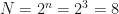
The state before the kickback:

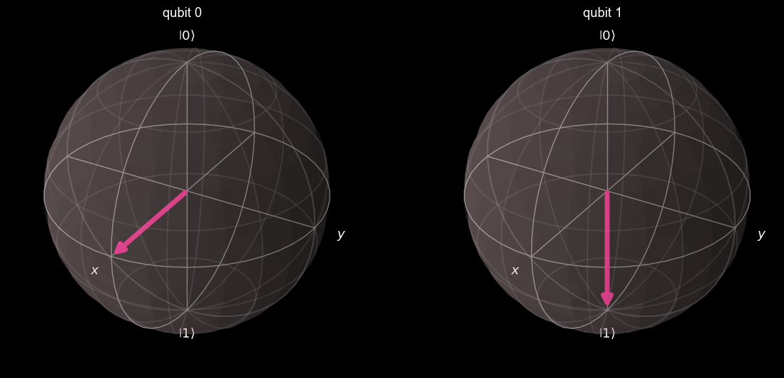
and the state after the kickback:

The control qubit (qubit 0) had its Bloch vector rotated around the $z$ -axis by an angle $\phi$ , even though we didn’t touch it; and the target qubit (qubit 1) did not move – although it still did acquire a global phase (which is physically unobservable). The target qubit is acting consistently with being an eigenstate of the rotation unitary.

The phase kickback trick works if the target qubit is an eigenstate of the controlled unitary, then the control qubit picks up a phase.

In fact, if the target qubit was not an eigenstate of the controlled unitary, then the controlled unitary would entangle both control and target qubit, and you would not achieve a clean phase kickback.

Conclusion

It turns out that many quantum algorithms boil down to somehow encoding the answer you’re looking for in to the phase of ancilla qubits (with the help of controlled-unitary gates). The generalised Hadamard maps $|x\rangle\mapsto|\tilde{x}\rangle$ with amplitudes $\omega^{xz}$ . These Fourier basis states $|\tilde{x}\rangle$ are eigenstates of the “shift” unitary $U_a|z\rangle = |z + a\mod N\rangle$ in an $N$ -dimensional computation basis $|z\rangle,\, z \in \{0,1,\dots, N-1\}$ , with eigenvalues $\omega^{-xa}$ . A controlled shift acting on a target in $|\tilde{x}\rangle$ leaves the target unchanged but affects the control’s amplitude by $latex\omega^{-xa}$.

Thus, all the information about how many times (also the basis label) you applied the shift unitary $U_a$ becomes encoded in the phase of the control qubit!

References

[1] https://medium.com/quantum-untangled/a-clever-quantum-trick-54f27e2518a4

[2] https://nosarthur.github.io/quantum%20information%20and%20computation/2018/01/26/kickback.html

[3] Quantum Phase Estimation – Qiskit Textbook

[4] Quantum Algorithms Revisited – Cleve, Ekert, Macchiavello & Mosca (1998).+

[5] Phase Kickback | QuTech Academy – Ben Criger (2018)

	Muhammad Shumail on Hadamard & CNOT
	spiral on A Recipe for Pricing
	Deutsch-Jozsa Algori… on Quantum Oracles
	Raymond Glowner on Fractal Manifolds III –…
	Parvez on A Recipe for Pricing

From First Principles

Mathematics Without Hand Waving

The Phase Kickback Trick

Introduction