Feynman-Kac in SageMath

In the previous few posts, we have been building up a small stochastic-calculus library on top of SageMath in Python. We have added extra operations and built new objects that allow us to represent Ito processes, Ito’s lemma, infinitesimal generators, the Kolmogorov equations, exponential martingales and, most recently, Girsanov’s theorem.

But I want to take a slightly different route in this post.

Rather than starting with stochastic differential equations and asking “what can we do with these?“, I want to strip things back and start with something much more basic and fundamental: a space of functions.

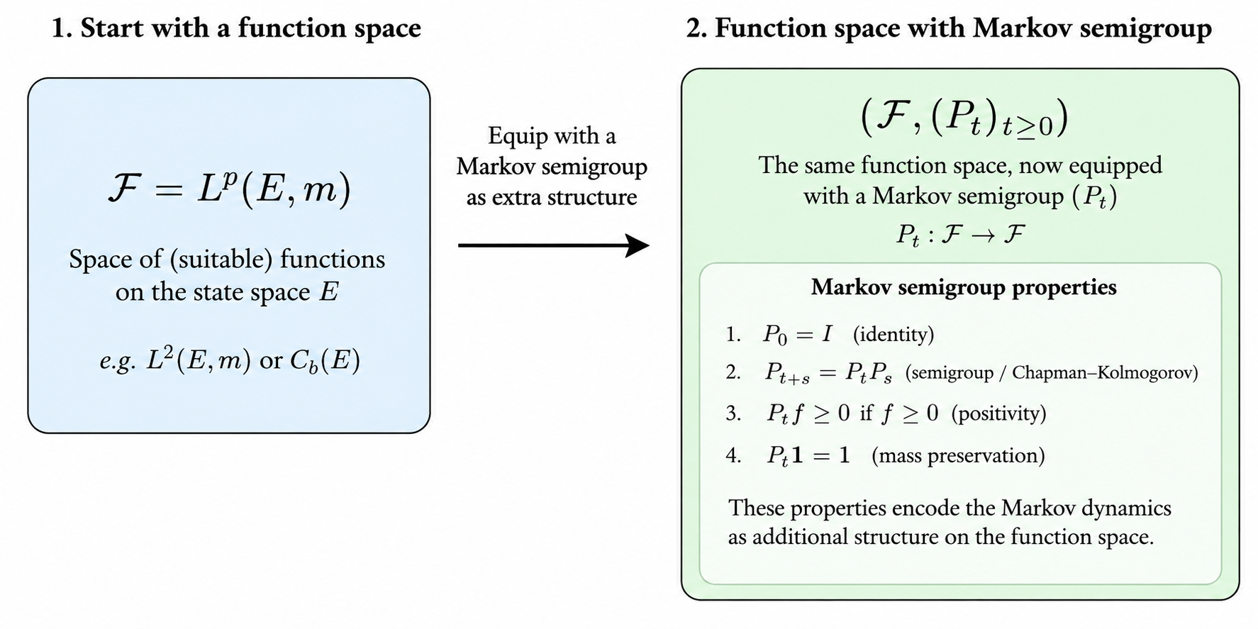
For intuition, imagine all we have is a function space such as , which denotes the space of square-integrable functions on the real line. This is essentially the SageMath library, which is exactly what we started with in Python.

At this point, there isn’t much going on, relatively speaking. We have functions, yes. We can differentiate and integrate them. We can add them together, and multiply them by scalars. But there is certainly no concept of, say, time evolution.

So let’s add some structure.

Adding Some Structure: the Markov Semigroup

Suppose is a time-homogeneous Markov process. If this process (sequence of random variables indexed by time ) is currently at the value , then after some elapsed time it will generally not be at one deterministic point. Instead, it has a probability distribution over possible future states. We describe this symbolically as a transition density: . Thus, for a fixed starting point and time , the function tells us the probability of finding the process in some infinitesimal region after evolving time .

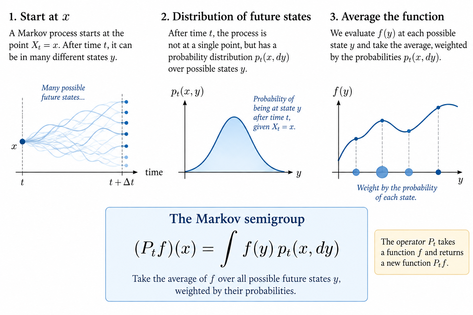
Now take one of the functions from our function space, or from SageMath Python.

We can use this transition function to construct a new function by averaging over all possible states that it could possibly reach in time. That is,

But this is an operator, so let us denote this operator by .

This operator acts on functions as inputs, and outputs another function (we don’t have a letter, so let us denote it by what has happened to the original) .

Now, this operator should look familiar to you: It is just the definition of an expectation: .

So the expectation has not been inserted into our space by magic, no. It appears naturally when we equip the space with the additional structure of a Markov semigroup. This (also known as a transitional kernel) supplies a probability distribution over future states, and we use the familiar operation of integration (it comes for free) to average over those states a return a new function.

Where does the Semigroup Property Come From?

We get this expectation operator for free, but calling the collection a semigroup requires more than simply having a family of operators. We need to show that they compose according to the specific rule:

But this is easy.

Suppose the process starts at and allow it to evolve over time , reaching some intermediate state , and then continue evolving for another amount of time until it reaches .

What is ? Well, now we need to take into account the extra information we get at time , so we need the tower rule, and so our conditional expectation becomes

Again, nothing special, we’ve just inserted an intermediate conditioning step.

But now we use the Markov property!

This is additional structure that we equip to our function space which says that, conditional on the present state , the future evolution after time does not depend on the path by which we arrived there. It is memoryless up to that point. Therefore,

Because we have assumed the process is time-homogeneous, the distribution of the process units after time , conditional on , is the same as the distribution units after time zero when starting from .

But that is precisely how we defined our transition operator .

Hence,

Substitute this back into the tower-property expression:

Now apply our definition of the operator again. Evolving the function for units of time gives

Therefore,

Since this holds for every suitable function , we have:

And so we have obtained the semigroup composition law without assuming it!

Showing the Markov Semigroup in Python

For a simple example, consider Brownian motion . We know that its Markov semigroup acts on a function according to

Then, since we can write the same operator as

So our apparently abstract operator is now actually quite concrete: it takes a function and averages it against the transition density of the Markov process.

For a simple polynomial such as our usual test one: we know immediately that

This gives us a particularly simple semigroup that we can represent directly in SageMath:

from sage.all import var, diff 
x, t = var("x t") 
f = x^2 
def brownian_semigroup_x2(f, x, t): 
  return x^2 + t 
  
Pt_f = brownian_semigroup_x2(f, x, t) 
print("f(x) =", f) 
print("P_t f(x) =", Pt_f)

We don’t necessarily code this into our Stochastic Calculus Python library. Instead we implement its infinitesimal shadow…

Zooming In: the Infinitesimal Generator

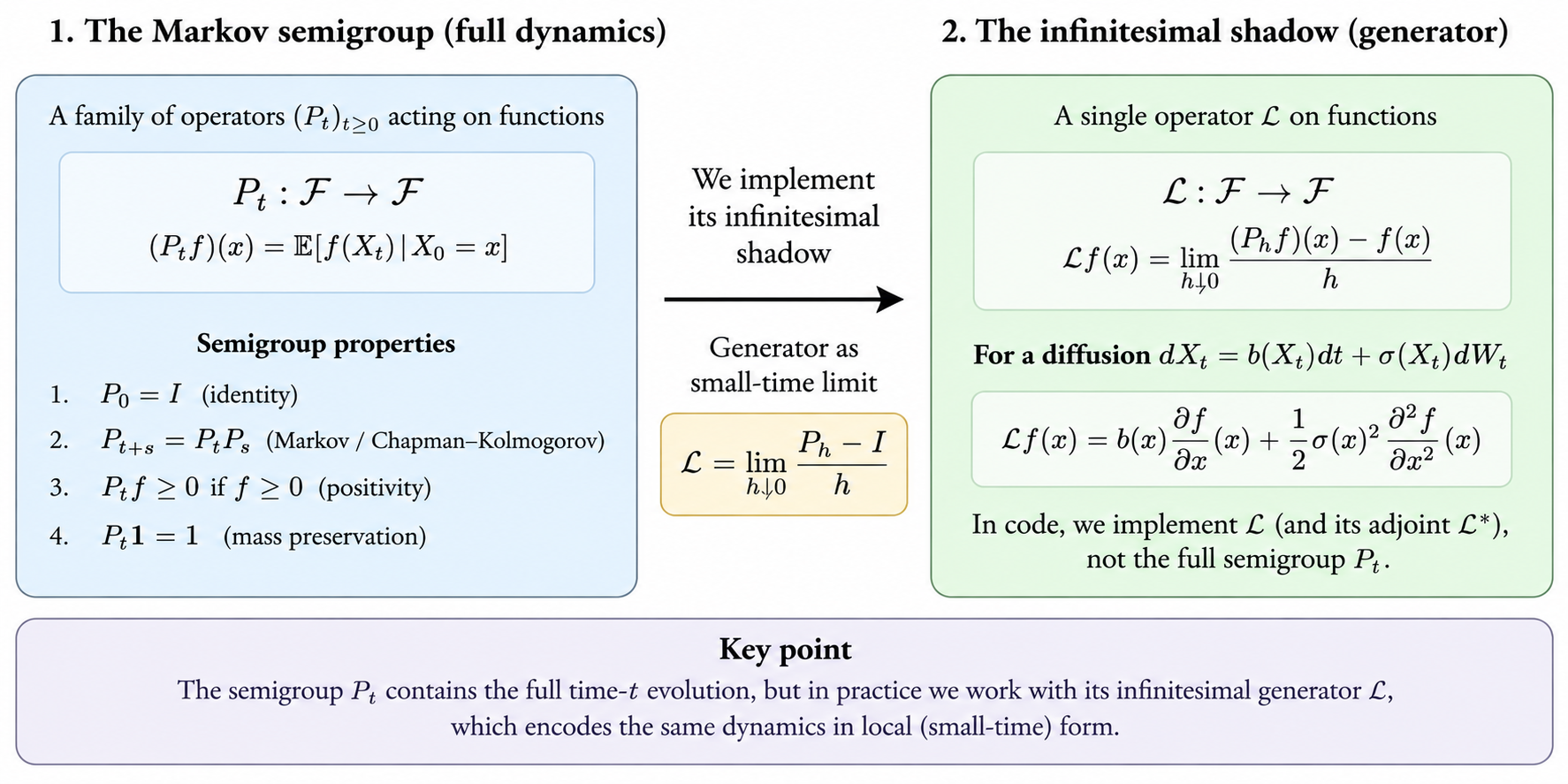
If tells us how a function from SageMath evolves over some finite period of time, a natural question to ask is: what is the instantaneous rate of that evolution? Can we even take a derivative of a semigroup at a point in time, say at ? We can and it is called the infinitesimal generator.

We implemented the infinitesimal generator into our code.

def generator(self, f, simplify_result: bool = True):
    fx = diff(f, self.x)
    fxx = diff(fx, self.x)
    expr = (
        self.drift * fx
        + SR(1) / SR(2) * (self.diffusion ** 2) * fxx
    )

This is exactly the infinitesimal generator of the standard diffusion

and we write it as

And this is the first important bridge.

The infinitesimal generator has not appeared as some arbitrary differential operator that we decided would be useful for stochastic calculus. It is the derivative of the Markov semigroup!

The semigroup describes finite-time evolution. The generator describes the infinitesimal evolution, and it is the infinitesimal evolution which we code up in Python.

And suddenly we have a PDE!

Now things start moving rather quickly.

If we define then the Markov semigroup tells us how evolves, while the infinitesimal generator tells us its instantaneous rate of change. Under the appropriate regularity conditions,

Therefore,

We have acquired a partial differential equation!

For Brownian motion this becomes the heat equation!

Nothing in our original blank canvas contained a heat equation. It appeared because we equipped our function space with a Markov evolution and then asked for its infinitesimal behaviour.

This is essentially the Kolmogorov backward equation in semigroup form.

Uncovering Hidden Duality

There is also a dual story.

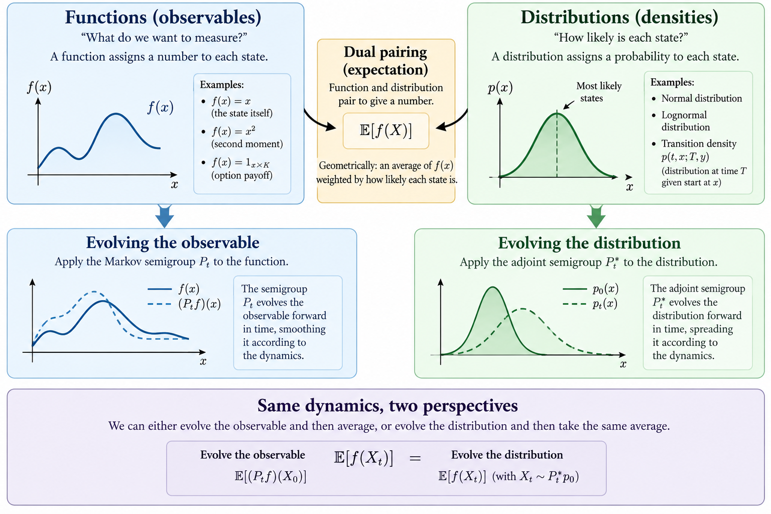
So far, our Markov semigroup acts on functions . We can think of a function as an observable: given the state , it tells us some quantity we would like to measure.

But there is another side to the story. Rather than evolving the observable, we could evolve the probability distribution of the state itself.

These two viewpoints meet with a handshake via the definition of the expectation:

Here, describes what we measure, while describes how likely the different, measurable states are.

The duality is between (observable, function) and (distribution). Combined under an integral, they form a single, real number, which we will denote by .

We already know that the Markov semigroup evolves observable functions. Is there an object, say which evolves distributions? There is, and it is precisely the object which produces the same real number except when it operates on the distribution instead of on the function, i.e. when operates on a distribution and evolves it forward through time via , giving:

Infinitesimally, these two, dual evolutions are governed by

And this is precisely where we get two Kolmogorov equations from!

The backward Kolmogorov equation describes the evolution of an observable function using the infinitesimal generator:

implemented in Python as

def generator(self, f, simplify_result: bool = True):
    fx = diff(f, self.x)
    fxx = diff(fx, self.x)
    expr = (
        self.drift * fx
        + SR(1) / SR(2) * (self.diffusion ** 2) * fxx
    )

The forward Kolmogorov equation (or Fokker-Planck equation) describes the evolution of the probability distribution using the adjoint infinitesimal generator:

This is precisely the distinction already represented in our SageMath implementation, where generator() constructs , and formal_adjoint_applied() constructs , and the corresponding functions construct the backward and forward Kolmogorov equations.

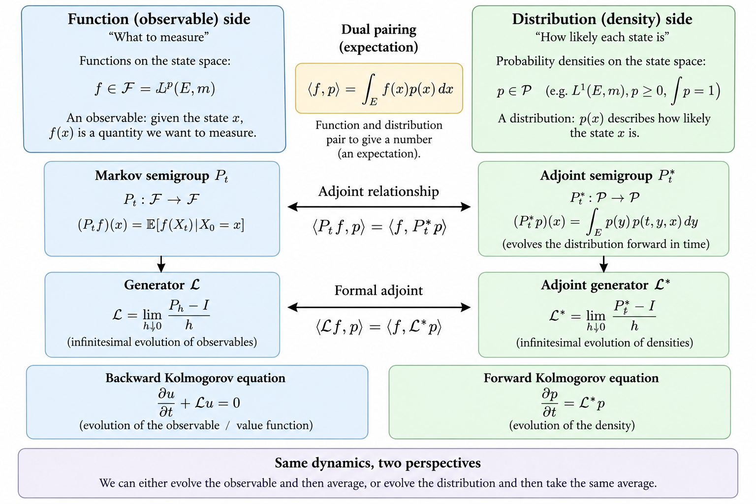
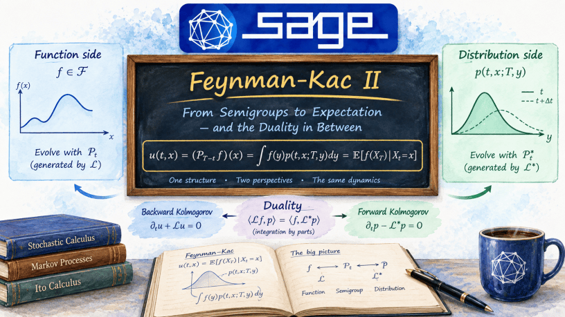
So the two sides of this illustration can be found in our code.

# Observable (LHS)
Lf = generator(f, state_vars, drift, diffusion)
# Distributrion (RHS)
Lstar_p = formal_adjoint_applied(p, state_vars, drift, diffusion)

Where is Feynman–Kac hiding?

There is one particularly interesting feature of the definition we started with:

But we have just discovered that this same object solves a PDE. So the same mathematical object can be viewed in two completely different ways.

On one side, is the solution of a partial differential equation generated by . On the other, is an expectation over paths of the underlying Markov process.

That is the door through which Feynman–Kac enters.

The relationship between PDEs and expectations is therefore not some miraculous identity dropped on us from above. We can see where it comes from, and we can code it up!

1. We started with a space of functions.
2. We equipped that space with a Markov semigroup.
3. The semigroup gave us an infinitesimal generator.
4. The generator gave us the Kolmogorov equations.
5. And the semigroup itself had been defined in terms of conditional expectations all along.

The PDE and the expectation have therefore been two descriptions of the same evolution from the beginning.

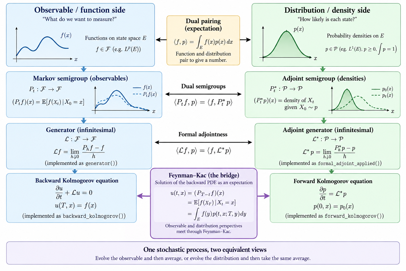
From the above image we can see the pieces and what they are implemented as. Down the left-hand “observable” side we see functions and the infinitesimal generator implemented as generator(). The dual “distribution” side has this implemented as formal_adjoint_applied(). Similarly, for the dynamics, the left-hand observable function side has the backward Kolmogorov equation implemented as backward_kolmogorov() and the dual distribution side has this implemented as forward_kolmogorov().

Conclusion

We started this post with almost nothing: just a space of functions and the operations that SageMath already gives us.

By equipping that space with the additional structure of a Markov semigroup, however, a large amount of stochastic calculus begins to emerge quite naturally.

The semigroup structure gives us a notion of finite-time evolution, its infinitesimal behaviour gives us a generator, and the dual notion gives us its adjoint. From these came the backward and forward Kolmogorov equations.

Feynman-Kac then ties this picture together.

We now see that the PDE, the conditional expectation, and the pairing between an observable function and a probability distribution is not three unrelated constructions. They are actually three views of the same underlying space and the objects therein.

Up Next

So far we have mostly exposed the mathematical structure. In the next post we will make it concrete.

Using a Jupyter Notebook and our stochastic calculus library, we will work through a complete Feynman-Kac example for geometric Brownian motion.

We will follow both sides of the dual picture we have illustrated in this blog, that is, showing the evolution of an observable function with the infinitesimal generator, and evolving the corresponding probability distribution with the adjoint, thereby verifying the backward and forward Kolmogorov equations, and finally bridging the two sides together through the handshake:

In other words, we will make Python do the handshake for us!

References

1. https://www.sagemath.org

Appendix

Implementation

IGenerator.py

from Ito.ito_algebra import Ito
from Ito.sde_transforms import extract_sde_coeffs
from Ito.generator import *
def generator_from_dX_1d(f, x, dX: Ito, dw_index: int = 1):
    mu, sigmas = extract_sde_coeffs(dX)
    sigma = sigmas.get(dw_index, 0)
    return generator_1d(f, x, mu, sigma)
def ito_operator_from_dX_1d(f, t, x, dX: Ito, dw_index: int = 1):
    mu, sigmas = extract_sde_coeffs(dX)
    sigma = sigmas.get(dw_index, 0)
    return ito_operator_1d(f, t, x, mu, sigma)
def generator_from_dX_scalar_multiW(f, x, dX: Ito):
    mu, sigmas = extract_sde_coeffs(dX)
    return generator_scalar_multiW(f, x, mu, sigmas)
def ito_operator_from_dX_scalar_multiW(f, t, x, dX: Ito):
    mu, sigmas = extract_sde_coeffs(dX)
    return ito_operator_scalar_multiW(f, t, x, mu, sigmas)

generator.py

from __future__ import annotations
# noinspection PyUnresolvedReferences
from sage.all import var, SR, diff, vector, matrix  # type: ignore
def gradient(f, vars_):
    return vector([diff(f, v) for v in vars_])
def hessian(f, vars_):
    return matrix([[diff(f, vi, vj) for vj in vars_] for vi in vars_])
def generator_1d(f, x, mu, sigma):
    """
    Spatial generator for 1d Ito diffusion:
        dX = mu(t,x)dt + sigma(t,x)dW
        L[f](x) = mu f_x + 1/2 sigma^2 f_xx
    """
    fx = diff(f,x)
    fxx = diff(fx,x)
    return mu * fx + SR(1) / SR(2) * (sigma ** 2) * fxx
def ito_operator_1d(f, t, x, mu, sigma):
    """
    Full Ito operator:
        (d/dt + L)[f]
    """
    ft = diff(f,t)
    return ft + generator_1d(ft, x, mu, sigma)
def covariance_from_sigmas(sigmas: dict):
    """
    Scalar-state, multi-W case:
        a = sum_i sigma_i^2
    """
    return sum(si ** 2 for si in sigmas.values())
def generator_scalar_multiW(f, x, mu, sigmas: dict):
    """
    Generator for scalar state driven by multiple
    independent Brownian motions.
    """
    fx = diff(f, x)
    fxx = diff(fx, x)
    a = covariance_from_sigmas(sigmas)
    return mu * fx + SR(1) / SR(2) * a * fxx
def ito_operator_scalar_multiW(f, t, x, mu, sigmas: dict):
    return diff(f,t) + generator_scalar_multiW(f, x, mu, sigmas)
def generator_L_1d(f, x, mu, sigma):
    fx = diff(f,x)
    fxx = diff(fx,x)
    return mu * fx + SR(1) / SR(2) * (sigma ** 2) * fxx
def ito_operator_L_1d(f, t, x, mu, sigma):
    ft = diff(f,t)
    return ft + generator_L_1d(f,x,mu,sigma)

kolmogorov.py

from __future__ import annotations
# noinspection PyUnresolvedReferences
from sage.all import var, SR, diff, matrix  # type: ignore
def ensure_list(x):
    return x if isinstance(x, list) else [x]
def covariance_from_diffusion(diffusion, n):
    """
    Convert diffusion specification into covariance matrix a = sigma sigma^T.
    Supported:
      - scalar expression for 1D
      - list of expressions for diagonal independent factors in 1D or componentwise
      - Sage matrix interpreted directly as covariance matrix if shape is n x n
      - rectangular sigma matrix, converted to sigma * sigma.transpose()
    """
    if hasattr(diffusion, "nrows") and hasattr(diffusion, "ncols"):
        if diffusion.nrows() == n and diffusion.ncols() == n:
            return diffusion
        return diffusion * diffusion.transpose()
    if n==1:
        diffs = ensure_list(diffusion)
        return matrix(SR, 1, 1, [sum(g**2 for g in diffs)])
    diffs = ensure_list(diffusion)
    if len(diffs) != n:
        raise ValueError("For multi-dimensional state, diffusion must be an n x n marix, or a length-n diagonal list!")
    sigma = matrix(SR, n, n, 0)
    for i in range(n):
        sigma[i, i] = diffs[i]
    return sigma * sigma.transpose()
def generator(f, state_vars, drift, diffusion):
    """
    Apply infinitesimal generator L to a test functional f.
    L[f](x) = sum_i b_i d_i f + 0.5 sum_{i,j} a_{ij} d_{ij} f
    :param f:
    :param state_vars:
    :param drift:
    :param diffusion:
    :return:
    """
    xs = ensure_list(state_vars)
    bs = ensure_list(drift)
    n = len(xs)
    if len(bs) != n:
        raise ValueError("Drift length must match number of state variables!")
    a = covariance_from_diffusion(diffusion, n)
    first_order = sum(bs[i] * diff(f, xs[i]) for i in range(n))
    second_order = sum(
        a[i, j] * diff(f, xs[i], xs[j])
        for i in range(n)
        for j in range(n)
    ) / 2
    return first_order + second_order
def formal_adjoint_applied(phi, state_vars, drift, diffusion):
    """
    Apply the formal adjoint L* to phi
    L*phi = -sum_i d_i(b_i phi) + 1/2 sum_{i,j} d_{ij}(a_{ij} phi)
    :param phi:
    :param state_vars:
    :param drift:
    :param diffusion:
    :return:
    """
    xs = ensure_list(state_vars)
    bs = ensure_list(drift)
    n = len(xs)
    if len(bs) != n:
        raise ValueError("Drift length must match number of state variables!")
    a = covariance_from_diffusion(diffusion, n)
    drift_term = -sum(diff(bs[i] * phi, xs[i]) for i in range(n))
    diffusion_term = sum(
        diff(a[i, j] * phi, xs[i], xs[j])
        for i in range(n)
        for j in range(n)
    ) / 2
    return drift_term + diffusion_term
def backward_kolmogorov(u, t, state_vars, drift, diffusion, simplify_result=True):
    """
    Returns the Backward Kolmogorov PDE expression:
    u_t + L u
    :param u:
    :param t:
    :param state_vars:
    :param drift:
    :param diffusion:
    :param simplify_result:
    :return:
    """
    expr = diff(u, t) + generator(u, state_vars, drift, diffusion)
    return expr.simplify_full() if simplify_result else expr
def forward_kolmogorov(p, t, state_vars, drift, diffusion, simplify_result=True):
    """
    Returns the Forward Kolmogorov PDE expression:
    p_t - L* p
    :param p:
    :param t:
    :param state_vars:
    :param drift:
    :param diffusion:
    :param simplify_result:
    :return:
    """
    expr = diff(p, t) - formal_adjoint_applied(p, state_vars, drift, diffusion)
    return expr.simplify_full() if simplify_result else expr