Introduction
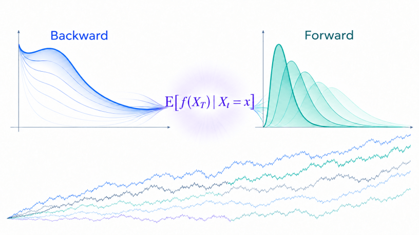
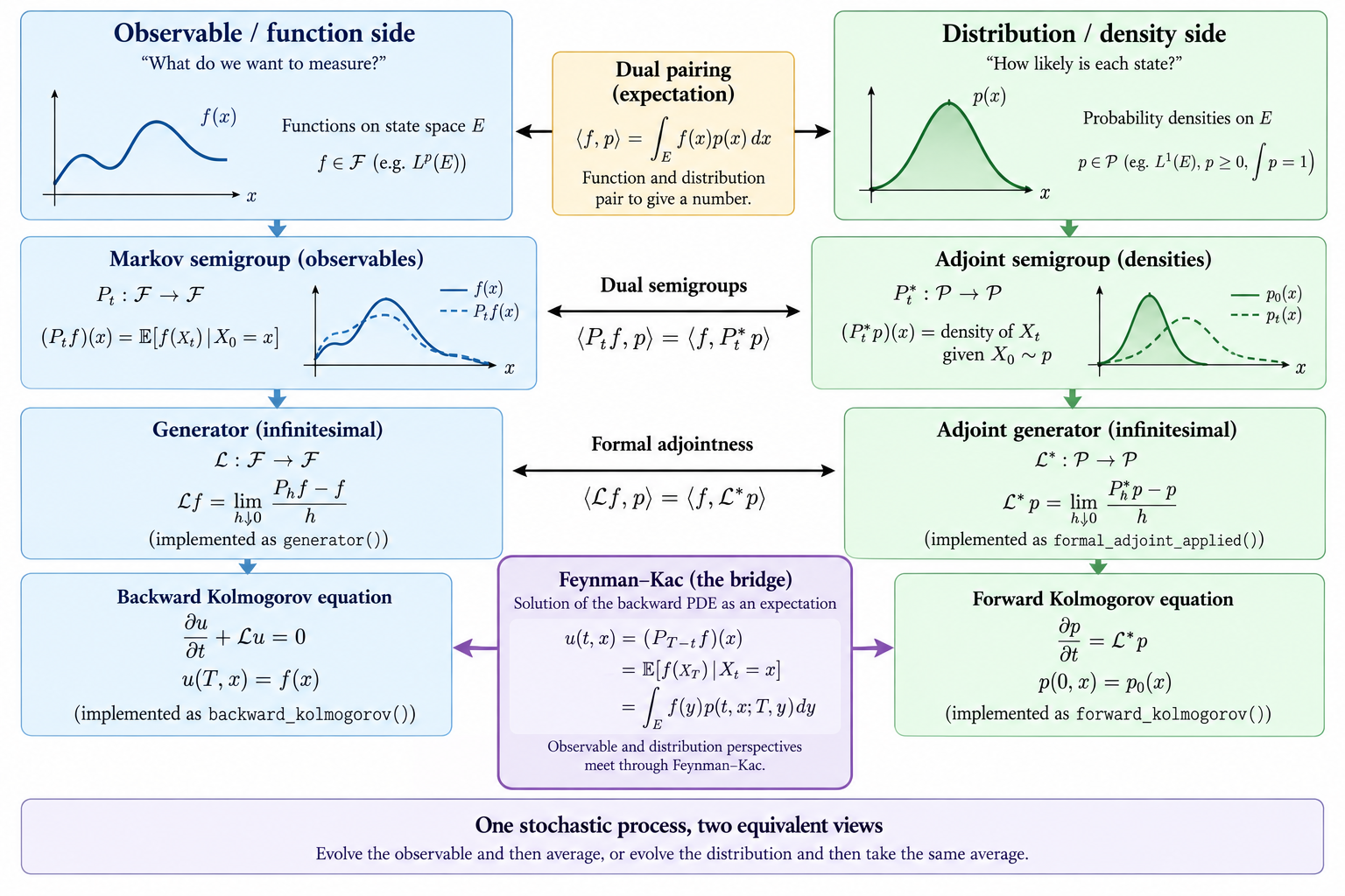
In the previous post, we introduced the Feynman-Kac equation by starting with a space of functions and equipping it with the Markov semigroup. From there, the infinitesimal generator and its adjoint gave us two (dual) ways to describe the same evolution of random information: we could evolve a function backward from a future observation (terminal boundary condition), or evolve some initial distribution forward. Then Feynman-Kac appeared where those two descriptions met.
This time, we will make it concrete in a SageMath Jupyter Notebook.
If the expectation is difficult but the PDE is tractable, then solve the PDE (usually numerically).
If the PDE is difficult, simulate paths ofand estimate the expectation by Monte Carlo.
We will use geometric Brownian motion and a simple function 

The aim here is to make this connection visible and practical, using only Python objects that we have already built. By the end, the backward PDE solution, the forward probability distribution, and the conditional expectation should really feel like three ways of looking at the same object.
Recall from the previous blog we ended with this picture:
Notebook Imports
Let’s first define these imports and helper functions.
# noinspection PyUnresolvedReferencesfrom sage.all import var, SR, exp, sqrt, latex, log, pi, assumefrom Sde.sde import SDE1D # type: ignorefrom Ito.ito_lemma import ito_lemma_1dfrom Ito.kolmogorov import backward_kolmogorovfrom IPython.display import display, Mathdef show_eq(lhs, rhs): display(Math(rf"{lhs} = {latex(rhs)}"))def show_text_math(text, expr): display(Math(rf"\text{{{text}}}\quad {latex(expr)}"))
Define the Markov Diffusion
We begin with geometric Brownian motion

Its future evolution depends on its current value, rather than the path it took to get there. This makes it a Markov diffusion. To see why, suppose we know that 


Recall from the previous post, that this lets us define a Markov operator 

 = \mathbb{E}\left[f(X_{t+s})\mid X_t=x\right]](https://s0.wp.com/latex.php?latex=%5Cdisplaystyle+P_s%5Bf%5D%28x%29+%3D+%5Cmathbb%7BE%7D%5Cleft%5Bf%28X_%7Bt%2Bs%7D%29%5Cmid+X_t%3Dx%5Cright%5D&bg=%23ffffff&fg=%23111111&s=0&c=20201002)
The infinitesimal generator 
 = \mu x f_x(x) + \frac12 \sigma^2 x^2 f_{xx}(x)](https://s0.wp.com/latex.php?latex=%5Cdisplaystyle%5Cmathcal%7BL%7D%5Bf%5D%28x%29+%3D+%5Cmu+x+f_x%28x%29+%2B+%5Cfrac12+%5Csigma%5E2+x%5E2+f_%7Bxx%7D%28x%29&bg=%23ffffff&fg=%23111111&s=0&c=20201002)
We represent the diffusion using our SDE1D class that we built earlier in this series:
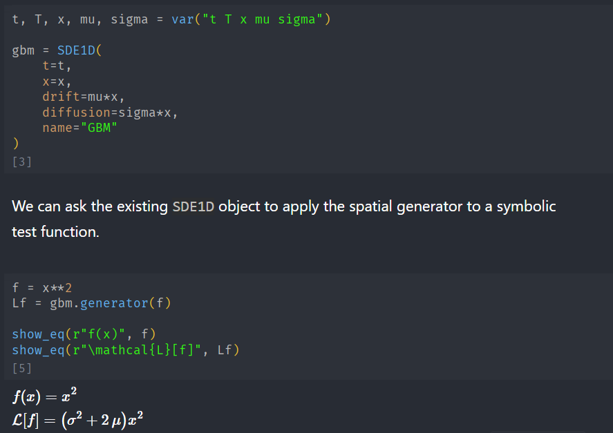
t, T, x, mu, sigma = var("t T x mu sigma")gbm = SDE1D( t=t, x=x, drift=mu*x, diffusion=sigma*x, name="GBM")
Now we choose the function we will follow for the rest of the notebook, SDE1D object to apply its spatial generator directly:
f = x**2Lf = gbm.generator(f)show_eq(r"f(x)", f)show_eq(r"\mathcal{L}[f]", Lf)
The result is
=(2\mu+\sigma^2)x^2](https://s0.wp.com/latex.php?latex=%5Cdisplaystyle%5Cmathcal%7BL%7D%5Bf%5D%28x%29%3D%282%5Cmu%2B%5Csigma%5E2%29x%5E2&bg=%23ffffff&fg=%23111111&s=0&c=20201002)
The generator has returned the instantaneous evolution of this observable function. The 

Next, we will turn this instantaneous description into a function that tells us the expected value of 

Compute the Conditional Expectation
Now that we have seen what the generator does to 
![[t,T]](https://s0.wp.com/latex.php?latex=%5Bt%2CT%5D&bg=%23ffffff&fg=%23111111&s=0&c=20201002)
Luckily for us, geometric Brownian motion has an exact transition formula. Conditional on 
![\displaystyle X_T=x\exp\left[\left(\mu-\frac12\sigma^2\right)(T-t)+\sigma\sqrt{T-t}Z\right]](https://s0.wp.com/latex.php?latex=%5Cdisplaystyle+X_T%3Dx%5Cexp%5Cleft%5B%5Cleft%28%5Cmu-%5Cfrac12%5Csigma%5E2%5Cright%29%28T-t%29%2B%5Csigma%5Csqrt%7BT-t%7DZ%5Cright%5D&bg=%23ffffff&fg=%23111111&s=0&c=20201002)
where 
The random variable 

![\displaystyle\mathbb{E}\left[X_T^2\mid X_t=x\right] = x^2 e^{(2\mu - \sigma^2)(T-t)}\cdot\mathbb{E}\left[e^{2\sigma\sqrt{T-t}Z}\right]](https://s0.wp.com/latex.php?latex=%5Cdisplaystyle%5Cmathbb%7BE%7D%5Cleft%5BX_T%5E2%5Cmid+X_t%3Dx%5Cright%5D+%3D+x%5E2+e%5E%7B%282%5Cmu+-+%5Csigma%5E2%29%28T-t%29%7D%5Ccdot%5Cmathbb%7BE%7D%5Cleft%5Be%5E%7B2%5Csigma%5Csqrt%7BT-t%7DZ%7D%5Cright%5D&bg=%23ffffff&fg=%23111111&s=0&c=20201002)
which simplifies to
![\displaystyle\mathbb{E}\left[X_T^2\mid X_t=x\right] = x^2 e^{(2\mu + \sigma^2)(T-t)}](https://s0.wp.com/latex.php?latex=%5Cdisplaystyle%5Cmathbb%7BE%7D%5Cleft%5BX_T%5E2%5Cmid+X_t%3Dx%5Cright%5D+%3D+x%5E2+e%5E%7B%282%5Cmu+%2B+%5Csigma%5E2%29%28T-t%29%7D&bg=%23ffffff&fg=%23111111&s=0&c=20201002)
where in this last line, we used the standard Normal identity ![\mathbb{E}[e^{aZ}] = e^{a^2 / 2}](https://s0.wp.com/latex.php?latex=%5Cmathbb%7BE%7D%5Be%5E%7BaZ%7D%5D+%3D+e%5E%7Ba%5E2+%2F+2%7D&bg=%23ffffff&fg=%23111111&s=0&c=20201002)
Let us call this conditional expectation 
tau = T - tu = x**2 * exp((2*mu + sigma**2) * tau)show_eq(r"u(t,x)", u)
The variable tau (or sometimes I use 

Before checking any PDE, we should first check what happens at the terminal time. When 


terminal_residual = (u.subs(t=T) - f).simplify_full()show_eq(r"u(T,x)", u.subs(t=T))show_eq(r"u(T,x) - f(x)", terminal_residual)assert terminal_residual == 0
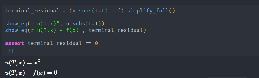
SageMath returns zero for the residual!
We have now constructed
The next question is whether this same function also solves the backward Kolmogorov PDE.
Verify the Backward Kolmogorov PDE
We obtained
For our geometric Brownian motion, we showed in a previous blog that the backward Kolmogorov equation is

with terminal condition 
The spatial terms are precisely ](https://s0.wp.com/latex.php?latex=%5Cmathcal%7BL%7D%5Bu%5D%28x%29&bg=%23ffffff&fg=%23111111&s=0&c=20201002)

Why the plus sign when we are working backward? The terminal time 

Our backward_kolmogorov() method now computes the left-hand side of the above PDE. If the conditional expectation we found really solves it, then the result should simplify to zero:
pde_residual = backward_kolmogorov( u=u, t=t, state_vars=x, drift=mu*x, diffusion=sigma*x, simplify_result=True)show_eq(r"u_t+\mathcal{L}[u]", pde_residual)assert pde_residual == 0
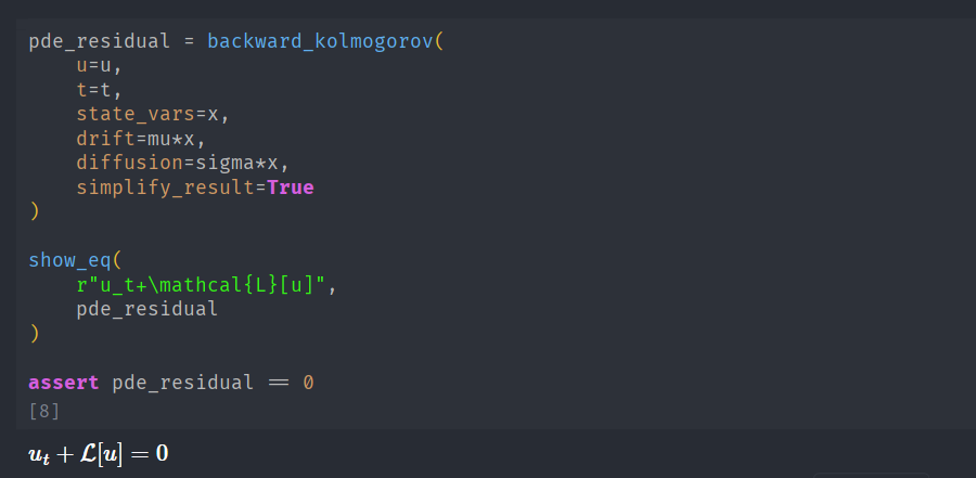
And it does!
We can check the same calculation through our SDE1D object, whose Ito operator applies 
sde_operator_residual = gbm.ito_operator(u)show_eq( r"(\partial_t+\mathcal{L})[u]", sde_operator_residual)assert sde_operator_residual == 0
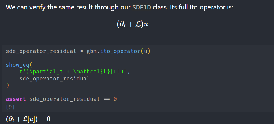
And as we can see, both routes give zero!
Thus, together with the terminal condition, this confirms that the function we calculated as ![\mathbb{E}[X_T^2 \mid X_t = x]](https://s0.wp.com/latex.php?latex=%5Cmathbb%7BE%7D%5BX_T%5E2+%5Cmid+X_t+%3D+x%5D&bg=%23ffffff&fg=%23111111&s=0&c=20201002)
Before turning to the dual, forward picture, let us see why the backward PDE produces a conditional expectation.
The Martingale Step: Applying Ito’s Lemma to the PDE Solution
We have checked that
To see this, let’s apply Ito’s lemma to 
\right)dt + \sigma X_t u_x dW_t](https://s0.wp.com/latex.php?latex=%5Cdisplaystyle%5Cleft%28u_t+%2B+%5Cmathcal%7BL%7D%5Bu%5D%28x%29%5Cright%29dt+%2B+%5Csigma+X_t+u_x+dW_t&bg=%23ffffff&fg=%23111111&s=0&c=20201002)
The expression multiplying 

We can see this cancellation using our Ito layer built earlier in this series:
du = ito_lemma_1d( f=u, t=t, x=x, dX=gbm.dX(), dw_index=gbm.dw_index)print("Itô differential of u(t, X_t):")print(du)show_eq(r"\text{drift}[du]", du.b)show_eq(r"\text{diffusion}[du]", du.c[gbm.dw_index])assert du.b.simplify_full() == 0
And the drift simplifies to zero as expected!
The remaining diffusion coefficient is

The zero drift tells us that 


![\displaystyle u(t,x)=\mathbb{E}\left[u(T, X_T) \mid X_t=x \right]](https://s0.wp.com/latex.php?latex=%5Cdisplaystyle+u%28t%2Cx%29%3D%5Cmathbb%7BE%7D%5Cleft%5Bu%28T%2C+X_T%29+%5Cmid+X_t%3Dx+%5Cright%5D&bg=%23ffffff&fg=%23111111&s=0&c=20201002)
At the terminal time, 
![\displaystyle u(t,x)=\mathbb{E}[X_T^2\mid X_t=x]](https://s0.wp.com/latex.php?latex=%5Cdisplaystyle+u%28t%2Cx%29%3D%5Cmathbb%7BE%7D%5BX_T%5E2%5Cmid+X_t%3Dx%5D&bg=%23ffffff&fg=%23111111&s=0&c=20201002)
This gives us the mechanism behind the expectation-to-PDE connection: the backward equation cancels the drift in Ito’s lemma, and the martingale property carries the terminal value back to time
We have now completed the observable side of the picture. Next, we will turn to its dual: evolve the transition density forward using the adjoint 
Following the Dual Side
So far we have followed the observable 
This time, we keep the starting state
Let 


Consequently, the transition density is also well-known:

Here 

Now let’s create this density in SageMath:
s, y = var("s y")assume(x > 0, y > 0, s > 0, sigma > 0)log_return = log(y/x) - (mu - sigma**2/2)*sp = exp(-log_return**2/(2*sigma**2*s)) / ( y*sigma*sqrt(2*pi*s))show_eq(r"p(s,y\mid x)", p)
The above generator 

 = -\frac{\partial}{\partial y}(\mu y p) + \frac12\frac{\partial^2}{\partial y^2} (\sigma^2y^2p)](https://s0.wp.com/latex.php?latex=%5Cdisplaystyle%5Cmathcal%7BL%7D%5E%2A%5Bp%5D%28x%29+%3D+-%5Cfrac%7B%5Cpartial%7D%7B%5Cpartial+y%7D%28%5Cmu+y+p%29+%2B+%5Cfrac12%5Cfrac%7B%5Cpartial%5E2%7D%7B%5Cpartial+y%5E2%7D+%28%5Csigma%5E2y%5E2p%29&bg=%23ffffff&fg=%23111111&s=0&c=20201002)
Then, our existing forward_kolmogorov() functions computes the residual ![p_s - \mathcal{L}^*[p]](https://s0.wp.com/latex.php?latex=p_s+-+%5Cmathcal%7BL%7D%5E%2A%5Bp%5D&bg=%23ffffff&fg=%23111111&s=0&c=20201002)
from Ito.kolmogorov import forward_kolmogorovforward_residual = forward_kolmogorov( p=p, t=s, state_vars=y, drift=mu*y, diffusion=sigma*y, simplify_result=True).simplify_full()show_eq(r"p_s-\mathcal{L}^{*}p", forward_residual)assert forward_residual == 0
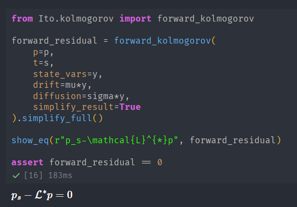
The above zero residual confirms that the density evolves forward according to the adjoint of the same generator we used on the backward side. Its initial condition is understood as a limit, i.e., as 
Bridging the Gap with the Handshake
We can now do the calculation promised at the start of the post. At elapsed time 

To evaluate the integral, use the change of variable

Under this substitution, 

![\displaystyle y^2 = x^2 \exp\left[2\left(\mu-\frac12\sigma^2\right)s + 2\sigma\sqrt{s}z\right]](https://s0.wp.com/latex.php?latex=%5Cdisplaystyle+y%5E2+%3D+x%5E2+%5Cexp%5Cleft%5B2%5Cleft%28%5Cmu-%5Cfrac12%5Csigma%5E2%5Cright%29s+%2B+2%5Csigma%5Csqrt%7Bs%7Dz%5Cright%5D&bg=%23ffffff&fg=%23111111&s=0&c=20201002)
The integral is therefore a normal exponential moment. Using the known identity: 

We can check that this result agrees with the conditional expectation constructed earlier:
density_moment = ( x**2 * exp(2*(mu - sigma**2/2)*s) * exp((2*sigma*sqrt(s))**2/2)).simplify_full()backward_value = u.subs(t=T-s)show_eq(r"\int_0^\infty y^2p(s,y\mid x)\,dy", density_moment)show_eq(r"u(T-s,x)", backward_value)handshake_residual = (density_moment - backward_value).simplify_full()show_eq(r"\text{difference}", handshake_residual)assert handshake_residual == 0
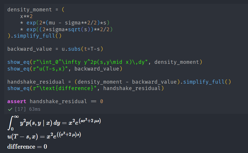
There is our long-awaited handshake! The difference is zero.
SageMath has confirmed that our analytically evaluated density integral equals the solution of the backward Kolmogorov equation (PDE). The forward equation evolves the density forward from the starting state, whilst the backward equation evolves the observable function backward from its terminal value. Pairing the density with that observable brings the two sides together:
![\displaystyle u(t,x) = \int_{0}^{\infty} y^2 p(T-t,y\mid x)dy = \mathbb{E}\left[X_T^2 \mid X_t = x\right] = x^2 e^{(2\mu + \sigma^2)(T-t)}](https://s0.wp.com/latex.php?latex=%5Cdisplaystyle+u%28t%2Cx%29+%3D+%5Cint_%7B0%7D%5E%7B%5Cinfty%7D+y%5E2+p%28T-t%2Cy%5Cmid+x%29dy+%3D+%5Cmathbb%7BE%7D%5Cleft%5BX_T%5E2+%5Cmid+X_t+%3D+x%5Cright%5D+%3D+x%5E2+e%5E%7B%282%5Cmu+%2B+%5Csigma%5E2%29%28T-t%29%7D&bg=%23ffffff&fg=%23111111&s=0&c=20201002)
Conclusion
We started with a question about a future observation: if geometric Brownian motion is at 
In the middle, we used Ito’s lemma and explained the link between those calculations. When we evaluate 

Finally, we also reached the answer from the other direction. Starting at 
That is the Feynman–Kac handshake made concrete in this simple example.
backward_value = u.subs(t=T-s)handshake_residual = (density_moment - backward_value).simplify_full()assert handshake_residual == 0
Our Ito and Sde Python Layer
The SageMath calculations are possible because of our Ito and Sde Python layers we built throughout this series. The class object SDE1D holds the GBM coefficients and applies its generator; backward_kolmogorov() and forward_kolmogorov() turn the generator and its adjoint into PDE residuals; and ito_lemma_1d() exposes the drift and diffusion terms when we need to evaluate
Why is it Useful to Have the Dual Representation?
In the end, we often have these types of equations: conditional expectations:
![u(t,x) = \mathbb{E}[g(X_t)\mid X_t = x]](https://s0.wp.com/latex.php?latex=u%28t%2Cx%29+%3D+%5Cmathbb%7BE%7D%5Bg%28X_t%29%5Cmid+X_t+%3D+x%5D&bg=%23ffffff&fg=%23111111&s=0&c=20201002)
and this is often very hard to calculate. But now we know that this is only one way to look at the solution. Feynman-Kac gives us an alternative route: solve the backward PDE with terminal boundary condition 
But it’s useful in both directions.
If the expectation is difficult but the PDE is tractable, then solve the PDE (usually numerically).
If the PDE is difficult, simulate paths of
In either case, the result is a function

