In this article we’re going to talk about tensors. They’re not too difficult to understand, especially if you know what a functional is, but often their representation can be awkward. So we’re going to start with the basics and slowly work up to the definition of an actual tensor. We’ll start with a short overview of vector spaces and their duals (when you have one you always have the other). We will then talk about adding extra structure to our space by way of including the set of all homomorphisms between vector spaces. We will certainly need this extra structure to be able to talk about maps between spaces, and the origination of these maps is not always obvious. Finally, we focus our attention on the maps which take you from vector spaces (or the dual) to the underlying field of numbers (or scalars). These maps (also called functionals) are the simplest type of tensor. From here is is but a short leap of faith to consider functionals which take you from, not one, but many vector spaces and duals to the underlying field of scalars.
Some people say that tensors are the workhorse of general relativity. Why is that? Why are they workhorses? In my opinion there are two reasons: First, because General Relativity, like all physical theories, is a framework used to measure stuff. When you measure something you would like to get a number back representing the value of your measurement. Measuring a thing should always result in a number; this number can then used to compare to other numbers (other measurements) and arrive at an opinion about the thing that you are measuring. A tensor is useful here because they always return a number. Always. But hang on, aren’t there other mathematical objects that return numbers? What makes tensors so special? Tensors are really, really good at converting many types of physical objects (things which can be described by vectors and covectors) in to numbers. They also behave very nicely when you change coordinate systems, something which physicists tend to do a lot. Furthermore, when a basis is present, tensors can also be neatly described by arrays or matrices of ordinary numbers, making it even easier to use them! And this is why tensors are workhorses.
If you want to get in to a bit more detail, tensors are also sensitive to curvature. It does this because they can have extra components that keep track of tiny differences between distances as measured on the curved surface and distances measured as if they were on a flat surface. Ordinary vectors just can’t do this.
But what’s so special about curvature? Well, for starters, ordinary classical calculus hates curved things. Then, to make matters worse, in the early 20th century Einstein proposed that gravity was a manifestation of curved spacetime (and not a flat force field emitted by an object with mass). This appeared like a great idea but calculus had to be re-invented for curved surfaces, and the tensor was born (with the help of Tullio Levi-Civita and Gregorio Ricci-Curbastro).
Vector Spaces
But before we get in to curved spacetimes, let’s go back to the beginning. Suppose you have two vector spaces 


If we have two vector spaces 


Note that 


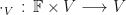
which maps the pair like so 


and so it takes vectors and maps them according to 
Linearity
We impose a condition on these maps to ensure that when you scale the vectors before the mapping, the resultant vector is also scaled by an associated amount – this makes the map a linear map and it satisfies

For convenience I’ve re-labelled the 


However, the 


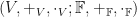
The point here is that writing a simple expression such as that of linearity of maps involves quite a bit of thinking about where you are and what operation you are using. Recall that with vector spaces you actually get quite a lot of structure! Not only do you get a set of vectors

but, don’t forget, you also get the addition and product operations that come with the underlying field! That’s two more types of addition and multiplication! We can see these in action. Consider the expression 


In light of this, we can no longer say “a vector space” because now we have to be specific about the underlying field, thus we say a
Dual Vector Spaces
So we are halfway there. We’ve introduced vector spaces, their underlying fields, and a bit of extra structure (a new set) containing all the homomorphisms from one vector space to another different vector space. Note that the addition and scalar multiplication operations are also maps but they live in a different set called the set of endomorphisms (or 
So the set 


Unfortunately, functionals require a bit of work to define. The reason being is that a vector is an object, but a number is a number, two very different things. The homomorphisms and endomorphisms were easy to define because we were mapping apples to apples and oranges to oranges. How do we turn a vector in to a number!? Gosh.
Basis
To answer the question we need a basis. A basis is even more structure we need to add to our vector space and it is, yet another, set. If we impose a basis on our vector space then we have an additional set of privileged vectors, let’s call them 


Now we see why we wrote the basis vectors with the index as a superscript! The Kronecker delta must be written with an index upstairs and downstairs; and downstairs is reserved for the basis vector index so the dual basis vector index goes upstairs (there’s also the Einstein summation convention to worry about, later).
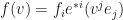
Just like a vector can be written in terms of its basis vectors, here’ one:

where the basis coefficients 

where the dual basis coefficients 
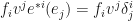
The final ingredient to see how functionals (dual vectors) turn vectors in to numbers is to now consider (in terms of basis) what happens when a dual vector eats a vector. First we write out the action in terms of basis vectors:
That was easy. Now by virtue of linearity let’s re-arrange:

But we know that when a dual basis vector eats a regular basis vector we get the Kronecker delta, so:
The Kronecker delta just equals 1 when 

These guys are numbers from the underlying field 

Side note: If we denote by 


Tensors
We have now met maps which take vectors to the field and called them dual vectors (or functionals), 
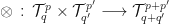
We are asking if we can define something that look like this:

In a way, this is like a super multiple version of an inner product. Instead of taking just one dual and one vector and getting a number back, you can take multiple duals and multiple vectors and get a number back. The above object is called a 
A (0,1)-tensor maps a vector to a real number, i.e. 


The set of all 
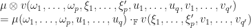
Thus, given a 


Tensor Basis
A tensor can be represented by its basis vectors (the basis vectors, obviously, they come from the associated dual and vector spaces) in the following way

Tensor Space
Let us collect together all 


References
Lecture 8: Tensor space theory I – Frederic P. Schuller
Nakahara, M. 2008 Geometry, Topology and Physics ed. II, Institute of Physics ISBN 0-7503-0606-8

Great explanation. I especially like how you explicitly identified the set of all objects of each particular type of object you introduced.