In the last article we were able to set up and configure our coding environment in Linux Ubuntu running Python 3, PyCharm, and venv, from a VirtualBox virtual environment. We have Qiskit pip-installed, running Git, and connected to our Quantum GitHub repository.

In this article, we are going to resume working out of our Quantum GitHub repo, adding a new Python file, checking it in, and importing the basics to be able to generate a very simple quantum circuit on two qubits.

We will run the circuit/algorithm on a simulator (not a real quantum computer), time the algorithm, and measure and plot the results using matplotlib.

This basic circuit will reveal some very interesting and unexpected quantum results.

Introduction

Let us begin by creating a brand new Python file in PyCharm within our Quantum virtual environment. Recall that we first check that we are in our virtual environment by going File > Settings, then under Project on the left hand side menu, expand the Project Interpreter. On the right hand side, up the top, you should see Python 3.6 (Quantum) ~/py_envs/Quantum/bin/python3 next to the Project Interpreter like so:

Right click the Project header > New > Python File. Call it testQiskit.py. We will begin this file with the following includes:

 import matplotlib as mpl
mpl.use('TkAgg')
import matplotlib.pyplot as plt
from qiskit import (QuantumCircuit, execute, Aer)
from qiskit.visualization import plot_histogram 

Under this, let’s define a new function that handles the figure showing:

 def show_figure(fig):
   new_fig = plt.figure()
   new_mngr = new_fig.canvas.manager
      new_mngr.canvas.figure = fig
      fig.set_canvas(new_mngr.canvas)
      plt.show(fig) 

Setting the Backend to be a Simulator

For now, and especially for testing, we want to run on IBM’s quantum simulator, not the real thing. This is good practice and besides compute time on the actual quantum computer is very limited.

To tell your program to run on the simulator we use the get_backend function from the Aer library.

 # Use Aer to set Backend to Simulator:
simulator = Aer.get_backend('qasm_simulator') 

The Qiskit Backend is one of three parts of the backend framework. The other two being  the provider and the job. The backend is the thing that runs the quantum circuit, while the provider accesses the backend and provides the backend objects to the interface, while the job keeps track of the submitted job.

Therefore, you would typically code something like get_backend('backend') in to the Qiskit Provider object, which then calls the underlying transpiler which compiles the submitted circuit in to a lower level language called the Qobj, a.k.a. the quantum object, which then provides an object to the Backend object to run. Finally, the Job object returns the result.

We prefer to use the Aer interface to the Provider.

Let’s see if we can list all the available backends from IBMQ: I’m going to quickly create a new Python file called testBackends.py. We will only need Qiskit.Aer for this quick exercise, so let’s write from qiskit import Aer. This little program will loop through all available backends and print them to the console:

 for backend in Aer.backends():
   print(backend.name()) 

Here is the output:

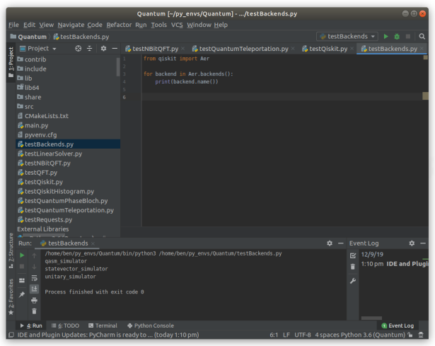
As you can see, running this little program produces three results:

• qasm_simulator
• statevector_simulator
• unitary_simulator

The QASM Simulator is a Qiskit Aer backend that supports multiple simulation methods and configurable options for each method. The QASM Simulator is an excellent place to start programming your first quantum programs. You can read more about it here.

Creating Your First Quantum Circuit

Let’s create a simple quantum circuit acting on a simple quantum register of 2 qubits. The Python object which instantiates a new circuit is the QuantumCircuit object. Let us declare it:

 # Create a Simple Quantum Circuit acting on a 2-qubit register:
circuit = QuantumCircuit(2,2) 

Here we have created a 2-qubit circuit with 2 classical bits (hence the (2,2) part).

Without knowing what does what, let us proceed blindly and add a Hadamard Gate to the first qubit (qubit 0), followed by a CNOT gate on the control qubit number 0 with target on qubit number 1. Finally, let us measure both qubits.

 # Add a Hadamard Gate on Qubit 0
circuit.h(0)
# Add a CNOT gate on control qubit 0 with target qubit 1:
circuit.cx(0,1)
$ Add measurements to each qubit at the end to convert in to classical bits:
circuit.measure([0,1],[0,1])  

We also want to use Matplotlib and our little custom function to plot the circuit. We do this by first creating a diagram (for MatplotLib to plot):

 diagram = circuit.draw(output='mpl')
show_figure(diagram) 

Saving and running the file produces the following circuit diagram

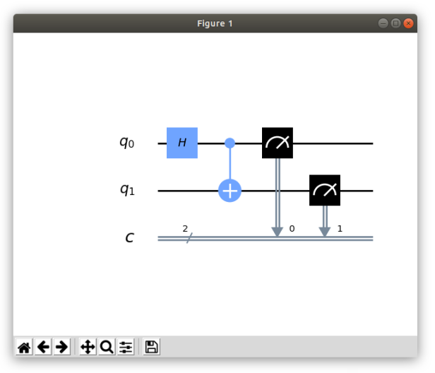
As you can see, the circuit object kind of acts as an appender. Each subsequent call with an instruction on what to add to the circuit simply appends the instruction to the end. Inserting new instructions or gates in between earlier pieces simply means scrolling up through your code and inserting a new circuit line.

Executing a Job on the Simulator

We will now execute the circuit. By executing a circuit we allow the qubits to evolve over time and through any logic gates that exist in the circuit. While we have no idea what this circuit does, our aim here is to see if we can just produce some measurements – we will worry about designing later.

We execute the quantum circuit using the execute object. This object requires three inputs:

• circuit,
• backend, and
• number of shots (or simulations)

We can immediately command PyCharm to execute the circuit with the following command:

 job = execute(circuit, simulator, shots=1000) 

Getting Results from a Job

As mentioned earlier, once a the job is executed we may retrieve results from it. This is done simply with the following command:

 result = job.result() 

This result is given to us as a huge array of 1,000 entries. Let us summarise the result by counting the number of times the qubits evolved in to one of the possible 4 results.

Since we started with 2 qubits, they can evolve in to $latex2^2 = 4$ possible states, namely:

• 00
• 01
• 10
• 11

When we measured the register at the end, across both qubits, we are essentially measuring simulation in to exactly one of these possible end states. However, since we are dealing with a quantum system, it is likely that we will get a different result every time we run it – quite unlike a classical circuit!

Let us see what we get with our very simple little circuit.

We will add in this code to count the final measurements and then use MatplotLib to plot the counts as a histogram.

 counts = result.get_counts(circuit)
plot_histogram(counts)
show_figure(plot_histogram(result.get_counts(circuit)))) 

Before we run the output, let us first try to guess what this circuit will do.

First of all, the Hadamard gate on the 1st qubit puts it in to a superposition, i.e. 50% of the time it will be measured to be in the 0 state and the other 50% of the time in the 1 state. At this point the 2nd qubit is in the default 0 state.

The CNOT gate comes along as says:

• if the 1st qubit (control) is a 0 and if the 2nd qubit (target) is a 0 then output 00.
• if the 1st qubit (control) is a 0 and if the 2nd qubit (target) is a 1 then output 01.
• if the 1st qubit (control) is a 1 and if the 2nd qubit (target) is a 1 then output 10.
• if the 1st qubit (control) is a 1 and if the 2nd qubit (target) is a 0 then output 11.

You can see wikipedia for the truth table here.

CNOT asks if the control qubit is a 1 then flip my state from 0 to 1 or from 1 to 0, else do nothing.

I have highlighted two scenarios in red which can not happen because the 2nd qubit (target) is initialised in the default 0 state and so can never be in the 1 state. So those two middle states above in red should never appear in any measurement.

Let’s see what happens:

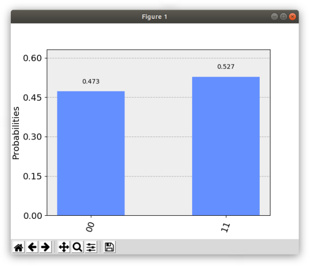
Perfect. We only see the 00 and the 11 state as predicted. However, those probabilities of measuring either state should be exactly 50% each!

Let’s increase the number of simulations from 1,000 to 100,000:

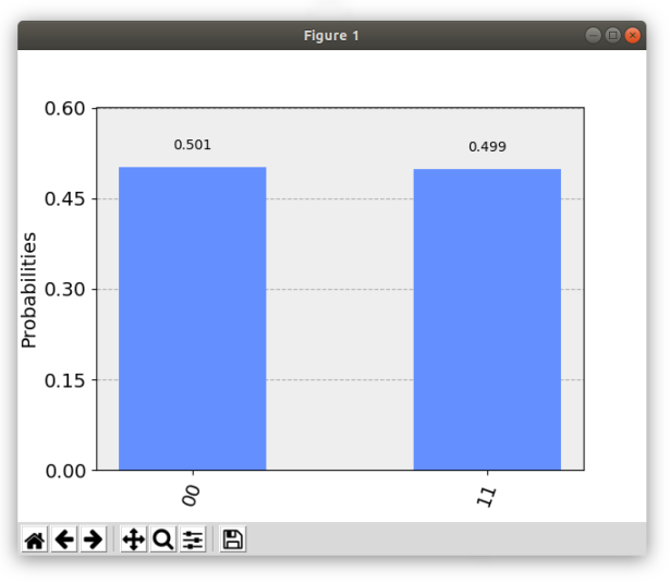
That’s better, but the program ran noticebly slower.

For 100,000 simulations the process took 0.276689 seconds, while for 1,000 simulations it only took 0.011332 seconds.

Entangled States

Of the four possible inputs (00, 01, 10, 11) we only get two outputs from this circuit: (00, 11). Why is this useful?

It turns out that this not only extremely useful but also superdense coding and quantum teleportation (which we will investigate in the next article).

Let’s look at the two qubits separately.

You run the circuit and observe the circuit. What do you see? Well, you see 0 50% of the time and 1 the other 50% of the time. A series of runs will see the values of 0 and 1 appearing at random, just like a classical bit undergoing a random change. Nothing crazy there.

Let’s look at the second qubit now. Again, you will see 0 50% of the time and 1 the other 50% of he time. A series of runs on the second qubit will see the values of 0 and 1 appearing at random, just like a classical bit undergoing a random change. Again, nothing crazy there.

Now let’s look at both qubits at the same time. Running the circuit multiple times will see both qubits returning a series of 0’s and 1’s at random. However, the two series of 0’s and 1’s will be exactly the same!

If it were two classical bits, this is what the output would look like:

q0 : 010110110010110110010110101
q1 : 110110010110101010110110010

If it is two qubits, the output would look like this:

q0 : 010110110010110110010110101
q1 : 010110110010110110010110101

See the difference?

The two qubits, although random in their individual measurements (horizontal numbers), are completely correlated (vertical numbers). We say that the two qubits are entangled.

The two qubits, although random in their individual measurements, are completely correlated with each other. We say that the two qubits are entangled.

I think this is truly remarkable. It is very counter-intuitive to think that one thing can generate a sequence of random 0’s and 1’s, and I mean truly random, while a second thing goes ahead and creates the exact same sequence of random 0’s and 1’s, without having to communicate or read any information from the first thing. In fact, this craziness is what prompted Einstein to investigate a Hidden-Variable theory to explain it. Hidden-variables were disproved in 1965 by John Bell.

What to do with Entangled Qubits?

It is clearly quite easy to entangle a pair of qubits, we just did it with a Hadamard Gate and a CNOT gate. But what to do with them? What is their power?

Suppose that someone on the street comes up to you with a sealed brown bag containing two marbles (you can feel them and hear them clinking around inside). Let’s also say that you are in the market for blue-coloured marbles (let’s say they are worth $1 each, more than red marbles, which are worthless; there aren’t any other colours). The man with the bag says that both marbles are indeed blue and asks for $2 for the bag.

Obviously you wouldn’t pay $2 for the bag without being certain that both marbles are blue. So you ask if you can check. The man says you can check one marble only, but you are allowed to manipulate the bag in any way that you wish.

Let’s say that you now simply reached your hand in and removed one marble to observe it and it was indeed blue, backing up what the man claimed. Would you still pay the $2?

Of course not. Only being allowed to check one of the two is not enough. There are four (equally likely, i.e. 25% each) outcomes you need to take in to consideration:

1. First marble is blue, second hidden marble is blue. Value = $1 + $1 = $2.
2. First marble is blue, second hidden marble is red. Value = $1 + $0 = $1.
3. First marble is red, second hidden marble is blue. Value = $0 + $1 + $1.
4. First marble is red, second hidden marble is red. Value = $0 + $0 = $0.

Since the first marble you drew was blue you must take in to account that second hidden marble could be red. The fair value of this deal (after first observing a blue marble) is, in fact, .

Note: the value of the marble bag before observing the first the marble is only .

So you haggle with the man and say that I only want to pay $1.50 for the two marbles. The man insists that both are blue and says that they are entangled marbles. How much do you pay now?

The answer is the full $2.00. Even if the odds that your first draw is blue was only 50%.

If the marbles are entangled their measurement results are perfectly correlated. So, if you observed a blue marble with your first pick, the second must also be blue.

What is the fair value of the entangled marble bag before drawing the first marble?

Before drawing you have a 50% chance of observing a red marble, but now there are only two outcomes to worry about:

1. First marble is blue, second hidden marble is blue. Value = $1 + $1 = $2.
2. First marble is red, second hidden marble is red. Value = $0 + $0 = $0.

Thus, the fair value is .

To summarise:

1. Fair value of classical bag before drawing = $1.00
2. Fair value of classical bag after drawing a blue marble = $1.50
3. Fair value of classical bag after drawing a red marble = $0.50
4. Fair value of entangled bag before drawing = $1.00
5. Fair value of entangled bag after drawing a blue marble = $2.00
6. Fair value of entangled bag after drawing a red marble = $0.00

Entangled qubits have the power to alter the underlying probability space, not the dynamics of the measurement process. This is an important property. It doesn’t suddenly make superposed qubit measurements non-random; they’re still definitely random. But it does alter the probability measure in the sense that now another qubit, still random, has a highly correlated outcome with respect to another qubit.

Summary

We have seen that two qubits can be entangled by first passing one qubit through a Hadamard gate (putting it in to a superposition of states with equally likely measurements) and then submitting it to a CNOT gate. The probably measure has been altered, and now the only non-zero probable outcomes are the 00 and the 11 state, equally likely.

Measuring one pair of an entangled pair immediately grants you knowledge of the state of the other qubit.

But doesn’t that mean you get two bits of information from measuring just one qubit? Is that free information?

Yes it is! And it’s called superdense coding.

In the next article we will investigate superdense coding further and actually run the code on a real quantum computer.

References

• Nielsen & Chuang, “Quantum Computing and Quantum Information“, Cambridge University Press (2016)
• Hidary, “Quantum Computing: An Applied Approach“, Springer (2019)
• Winston & Moreda, “Qiskit Backends: what they are and how to work with them“, http://www.medium.com (2018)
• Qiskit: www.qiskit.org.
• Quantum GitHub.